Chapter 16: The Cooke Triplet: Walking Through the Whole Computation Chain
A Cooke Triplet is a modest-looking lens.
Three elements. A positive element in front, a negative element in the middle, another positive element behind it. Compared with modern multi-element camera lenses, it looks almost simple.
That simplicity is exactly why it is useful here.
The Cooke Triplet is complicated enough to show real optical behavior:
- spherical aberration;
- coma;
- astigmatism;
- field curvature;
- distortion;
- chromatic correction;
- field-dependent image quality;
- optimization tradeoffs.
But it is still small enough that we can keep the whole design in view.
This chapter uses the Cooke Triplet as a full-chain example. We are not trying to teach every historical or commercial detail of triplet design. We are using it as a test bench.
Here we run the route this book has been building all along:
prescription
→ surfaces and materials
→ ray tracing
→ spot diagram
→ ray fan
→ OPD and wavefront
→ pupil function
→ PSF
→ OTF
→ MTF
→ merit function
→ optimization
→ before/after comparison
If the earlier chapters were individual tools on the table, this chapter is where we use them in sequence.
This is the check: when you see a final MTF curve, can you explain what had to happen before that curve existed?
By the end of this chapter, the answer should be yes.
One note before we start: this chapter uses one fixed teaching prescription instead of treating the Cooke Triplet as a vague placeholder. The numbers are intentionally rounded and pedagogical, not a claim about a historical patent or a production lens. That distinction matters. A fixed teaching prescription is enough to make the calculation chain inspectable. A production prescription would also need glass-catalog validation, tolerance analysis, manufacturability checks, and version-locked engineering review.
1. Why the Cooke Triplet is a good test case
A single thin lens is too simple for a full optical design story. It can show focal length and basic aberration, but it cannot carry much design tradeoff.
A complex modern photographic lens has the opposite problem. It may have many elements, aspheric surfaces, special glasses, floating groups, mechanical constraints, and proprietary design choices. It is realistic, but it is too much for a first full-chain walkthrough.
The Cooke Triplet sits in the useful middle.
It has enough degrees of freedom to make optimization meaningful:
radii
thicknesses
air spaces
glass choices
stop position
image plane position
It has enough aberration behavior to make analysis meaningful:
on-axis and off-axis spot diagrams differ
ray fans show structure
wavefront maps change across field
PSF changes with field and focus
MTF varies by field and direction
And it is small enough that we can still understand the prescription as a table.
That is why lens design education often returns to triplets. They are not toys. They are compact examples of real design logic.
For this book, the Cooke Triplet has one more advantage: it lets us demonstrate the educational value of an open computational workflow.
We can ask not only:
What is the MTF?
but also:
Which prescription produced it?
Which rays were traced?
Which field point was used?
Which wavelength was used?
Which wavefront became the pupil function?
Which PSF produced the OTF?
Which merit function changed the design?
That is the whole point.
2. What we will and will not do
This chapter is a walkthrough, not a full industrial lens design project.
We will not pretend that a few pages of code replace professional optical design software. We will not derive every third-order aberration term. We will not claim that a triplet optimized in a teaching script is ready for manufacturing.
What we will do is more focused:
take one complete lens
run the major analyses
connect each plot to its computational origin
perform a small optimization
compare before and after
That is enough to prove the main promise of the book.
We can now follow a lens from prescription data to image-quality metrics.
The Cooke Triplet is not the protagonist. The computation chain is.
3. The two-track approach in this chapter
We will keep the same two-track method used throughout the book.
Track A: minimal Python understanding
Track A is for understanding the skeleton. It uses small code fragments to show what kind of data is being passed around.
It does not implement a full production ray tracer here. We already built many of those pieces earlier:
- ray representation;
- surface intersection;
- vector refraction;
- pupil sampling;
- OPD to pupil function;
- PSF by FFT;
- OTF and MTF from PSF;
- merit function optimization.
In this chapter, Track A mostly reminds us what each stage means.
Track B: Optiland adapter boundary
Track B is not allowed to be a pile of almost-code. It needs a clean boundary. The book text should show the workflow; the companion code should lock the installed library version and implement a small adapter layer around the actual API.
Read Optiland examples in this chapter in one of two ways:
- Pure Python blocks are meant to be syntactically valid teaching code.
- Adapter sketches describe calls that must be implemented in the companion repository for the pinned Optiland version. They are marked as sketches rather than presented as directly runnable snippets.
A practical companion repository should include:
pyproject.toml
notebooks/16_cooke_triplet_full_chain.ipynb
src/optics_examples/cooke_triplet.py
src/optics_examples/analysis_adapters.py
tests/test_chapter_code_syntax.py
tests/test_cooke_triplet_smoke.py
The contract for the adapter is simple:
make_cooke_triplet()          -> optical system object
plot_layout(system)           -> layout figure or axis
run_spot_diagram(system, ...) -> spot data and figure
run_ray_fan(system, ...)      -> ray-fan data and figure
run_wavefront(system, ...)    -> OPD map, pupil mask, metadata
run_psf(system, ...)          -> PSF array, coordinate metadata
run_mtf(system, ...)          -> frequency axis and MTF curves
optimize_triplet(system, ...) -> optimized system and optimization log
This adapter does not hide the calculation. It prevents the printed book from depending on unstable method names while still requiring the companion code to prove the workflow.
4. The prescription: the lens as data
Before there are plots, there is a prescription.
A lens prescription is not merely documentation. It is the input data for computation.
A simplified triplet prescription might be represented as a table:
| Surface | Radius | Thickness to next | Material | Semi-aperture | Comment |
|---|---|---|---|---|---|
| 0 | Infinity | Object distance | Air | — | Object |
| 1 | Positive | Glass thickness | Crown glass | aperture | Front lens first surface |
| 2 | Negative | Air gap | Air | aperture | Front lens second surface |
| 3 | Negative | Glass thickness | Flint glass | aperture | Middle lens first surface |
| 4 | Positive | Air gap | Air | aperture | Middle lens second surface |
| 5 | Positive | Glass thickness | Crown glass | aperture | Rear lens first surface |
| 6 | Negative | Back focal distance | Air | aperture | Rear lens second surface |
| 7 | Infinity | — | Image | — | Image plane |
For this chapter, we use one fixed teaching prescription. The values below are rounded teaching values in millimeters. They are not presented as a historical Cooke patent prescription, and they are not a manufacturing prescription. Their job is to make the full computation chain concrete.
In code, it may look like this:
from dataclasses import dataclass
from typing import Optional


@dataclass
class SurfaceRecord:
    radius: float              # mm; use np.inf for plane
    thickness: float           # mm to next surface
    material_after: str        # material after this surface
    semi_aperture: float       # mm
    comment: str = ""


cooke_triplet_prescription = [
    SurfaceRecord(radius=  23.7, thickness=4.0,  material_after="CROWN", semi_aperture=8.0, comment="front element S1"),
    SurfaceRecord(radius= -80.0, thickness=6.0,  material_after="AIR",   semi_aperture=8.0, comment="front element S2"),
    SurfaceRecord(radius= -22.0, thickness=2.0,  material_after="FLINT", semi_aperture=6.5, comment="middle element S1"),
    SurfaceRecord(radius=  22.0, thickness=7.0,  material_after="AIR",   semi_aperture=6.5, comment="middle element S2"),
    SurfaceRecord(radius=  80.0, thickness=4.0,  material_after="CROWN", semi_aperture=7.5, comment="rear element S1"),
    SurfaceRecord(radius= -23.7, thickness=38.0, material_after="AIR",   semi_aperture=7.5, comment="rear element S2"),
]
These numbers are now the fixed teaching prescription for this chapter. A companion repository should keep the same table in machine-readable form, so every figure in this chapter can be regenerated from the same starting data.
The important point is this:
Every later plot begins from this kind of table.
A spot diagram is not drawn from nowhere. A wavefront map is not guessed. An MTF curve is not a software artifact.
They all start from surfaces, distances, materials, apertures, wavelengths, fields, and focus settings.
5. Building or loading the triplet in Optiland
In a pinned Optiland environment, you may either load a sample triplet or build one surface by surface.
The validated companion workflow looks like this:
# Validated wrapper workflow.
# Implemented for optiland==0.6.0 in the companion package.

optic = make_cooke_triplet()

plot_layout(optic)
If building manually, the conceptual steps are:
# Conceptual construction steps.

optic = OpticalSystem()

optic.add_surface(radius=23.7,  thickness=4.0,  material="CROWN", semi_aperture=8.0)
optic.add_surface(radius=-80.0, thickness=6.0,  material="AIR",   semi_aperture=8.0)
optic.add_surface(radius=-22.0, thickness=2.0,  material="FLINT", semi_aperture=6.5)
optic.add_surface(radius=22.0,  thickness=7.0,  material="AIR",   semi_aperture=6.5)
optic.add_surface(radius=80.0,  thickness=4.0,  material="CROWN", semi_aperture=7.5)
optic.add_surface(radius=-23.7, thickness=38.0, material="AIR",   semi_aperture=7.5)

optic.set_aperture(...)
optic.set_fields(...)
optic.set_wavelengths(...)
optic.set_image_plane(...)
The manuscript package implements the wrapper calls against optiland==0.6.0. If you port the example to another version, rerun the validation tests before trusting the plots.
The structure is what matters:
surfaces first
then aperture
then fields
then wavelengths
then image plane
then analysis
Do not start with MTF. Start with the lens.
6. Choosing fields and wavelengths
A lens does not have one universal performance value.
Performance depends on field point and wavelength.
For a simple triplet example, we might use three fields:
on-axis field
mid field
edge field
and three wavelengths:
blue
green
red
For example:
fields = [
    {"name": "axis", "angle_deg": 0.0},
    {"name": "mid",  "angle_deg": 7.0},
    {"name": "edge", "angle_deg": 14.0},
]

wavelengths = [
    {"name": "blue",  "wavelength_m": 486.1e-9, "weight": 1.0},
    {"name": "green", "wavelength_m": 587.6e-9, "weight": 1.0},
    {"name": "red",   "wavelength_m": 656.3e-9, "weight": 1.0},
]
These are the validation wavelengths used in this manuscript package. A different design goal may require different wavelengths or weights.
A monochromatic design problem is different from a polychromatic imaging problem.
An on-axis-only optimization is different from a field-wide optimization.
A slow lens is different from a fast lens.
So before running analysis, write down the configuration:
What field points?
What wavelengths?
What aperture?
What focus plane?
What performance target?
Without those answers, “the MTF of the lens” is an incomplete phrase.
A better phrase is:
the MTF of this lens at this field, wavelength set, aperture, focus, and direction
It is longer, but it is honest.
7. First plot: the layout
The layout is the first sanity check.
optic = make_cooke_triplet()

plot_layout(
    optic,
    fields=fields,
    wavelengths=wavelengths
)
A layout plot should answer basic questions:
- Are the surfaces in the expected order?
- Are the elements separated correctly?
- Is the stop where you think it is?
- Do rays pass through the clear apertures?
- Does the image plane look roughly plausible?
- Are there obvious ray failures?
The layout is not a performance plot. It does not prove the lens is good.
But it catches large modeling errors early.
If the layout is wrong, every later analysis is suspect.
A good habit is:
Never trust a spot diagram before looking at the layout.
Never trust an MTF curve before looking at the prescription and layout.
This may sound slow. It is faster than debugging a beautiful MTF curve from a broken model.
8. Paraxial check: focal length and f-number
Before real-ray analysis, check the paraxial skeleton.
A triplet is a real lens, but paraxial quantities still matter:
- effective focal length;
- back focal length;
- f-number;
- entrance pupil;
- image distance;
- approximate magnification if finite conjugates are used.
Validated wrapper call:
# Validated wrapper workflow for optiland==0.6.0.

paraxial = optic.paraxial_analysis()

print("Effective focal length:", paraxial.efl)
print("Back focal length:", paraxial.bfl)
print("F-number:", paraxial.f_number)
print("Entrance pupil diameter:", paraxial.entrance_pupil_diameter)
If your intended lens is around 50 mm focal length and the paraxial analysis says 5000 mm, do not continue to PSF.
The paraxial check is the system’s backbone.
It tells you whether the first-order behavior is roughly right before you ask about detailed aberrations.
This connects directly to Chapter 8:
paraxial optics is not old-fashioned decoration;
it is the first consistency check for the whole system.
9. Real ray tracing: where the geometry becomes honest
Now trace real rays.
In a full triplet, real rays do not obey the simple paraxial model exactly. They intersect curved surfaces at real points, refract using local surface normals, and accumulate errors.
Validated wrapper call:
# Validated wrapper workflow for optiland==0.6.0.

ray_bundle = optic.trace_rays(
    field=fields[1],
    wavelength=wavelengths[1],
    pupil_sampling="grid",
    num_rays=21,
)

print(ray_bundle.summary())
The real-ray trace is the engine behind many later plots.
From traced rays we can compute:
- spot diagram;
- ray fan;
- transverse aberration;
- chief ray behavior;
- vignetting;
- optical path length;
- wavefront error.
This is why the middle of the book spent so much time on rays.
If ray tracing is wrong, the later wave optics will not be trustworthy.
The computation chain depends on it:
prescription
→ surface intersections
→ refractions
→ ray bundle at image plane
That is the geometric foundation.
10. Spot diagram: the first image-quality view
The spot diagram is often the first visual performance check.
Validated wrapper call:
# Validated wrapper workflow for optiland==0.6.0.

spot_results = run_spot_diagram(
    optic,
    fields=fields,
    wavelengths=wavelengths,
    pupil_sampling="grid",
    num_rays=21,
)

spot_results.plot()
spot_results.report()
A spot diagram answers:
Where do traced rays land on the image plane?
For the triplet, you should expect field dependence.
The on-axis spot may be relatively compact. Off-axis spots may stretch, tilt, or grow. Different wavelengths may land in slightly different places or have different spreads.
This tells us several things:
- spherical aberration affects the on-axis spot;
- coma and astigmatism appear more strongly off-axis;
- chromatic aberration appears when wavelengths separate;
- focus choice changes the distribution.
But the spot diagram is still ray-based.
It does not show diffraction rings. It does not directly show MTF. It does not replace PSF.
Its role in the chain is:
real ray trace
→ image plane ray intercepts
→ spot diagram
It is a geometric image-quality view.
Useful, but not complete.
11. Reading the spot diagram without overreading it
A compact spot usually suggests better geometric imaging. A large spot suggests more blur.
But there are limits.
A small spot can still be larger than the diffraction-limited Airy disk. A spot smaller than the Airy disk may not matter much because diffraction dominates. A spot diagram near the diffraction limit can be less informative than wavefront, PSF, or MTF.
So for each field, compare spot size to the Airy scale.
A simple calculation:
def airy_radius_um(wavelength_m, f_number):
    return 1.22 * wavelength_m * f_number * 1e6


green = 587.6e-9
f_number = 4.0  # example; use paraxial result from the actual system

print("Airy first dark radius [um]:", airy_radius_um(green, f_number))
If the RMS spot radius is much larger than the Airy scale, geometric aberration dominates.
If the spot is comparable to or smaller than the Airy scale, diffraction analysis becomes especially important.
This is a good moment to remember one of the book’s recurring points:
Spot diagrams are computed results, not final truth.
They answer one question well. They do not answer every question.
12. Ray fan: structure inside the spot
A spot diagram shows where rays land. A ray fan shows how ray error changes across the pupil.
Validated wrapper call:
# Validated wrapper workflow for optiland==0.6.0.

ray_fan = run_ray_fan(
    optic,
    fields=fields,
    wavelengths=wavelengths,
    pupil_coordinate="normalized",
)

ray_fan.plot()
Ray fans are useful because they reveal structure.
A spot diagram might show a blur cloud. A ray fan can show whether the blur comes from:
- spherical-like behavior;
- coma-like asymmetry;
- astigmatic differences;
- chromatic separation;
- defocus;
- field-dependent imbalance.
This connects to Chapter 9.
A ray fan asks:
How does transverse ray error vary across the pupil?
For a triplet, compare the ray fan at different fields.
On-axis, the fan may show mostly symmetric aberration patterns.
Off-axis, the fan may become asymmetric or direction-dependent.
This is one reason the Cooke Triplet is a good teaching example. It is small, but not boring.
13. Wavefront and OPD: crossing from rays to phase
Now we move from ray intercepts to wavefront error.
The OPD map answers:
At each pupil point, how far ahead or behind is the real wavefront
compared with the reference wavefront?
Validated wrapper call:
# Validated wrapper workflow for optiland==0.6.0.

wavefront = run_wavefront(
    optic,
    field=fields[1],
    wavelength=wavelengths[1],
    pupil_sampling=128,
)

opd = wavefront.opd
mask = wavefront.pupil_mask

wavefront.plot_opd(units="waves")
wavefront.report()
The OPD is where the chain changes character.
The spot diagram and ray fan are geometric views. OPD prepares the system for diffraction calculation.
This is the bridge from Chapter 10:
real ray tracing
→ optical path length
→ reference wavefront comparison
→ OPD map
For the triplet, inspect OPD by field.
A good on-axis wavefront may be mostly symmetric. An off-axis wavefront may show coma-like or astigmatic structure. Different wavelengths may show different OPD behavior because refractive index changes.
This is not just another plot. It is the input to the pupil function.
14. Pupil function: encoding the wavefront as complex field
From OPD, we build the pupil function:
This is Chapter 11 returning inside a real lens workflow.
If the Optiland wavefront tool gives us OPD and a pupil mask, the teaching conversion is:
import numpy as np


def pupil_function_from_opd(opd, mask, wavelength, amplitude=None):
    if amplitude is None:
        amplitude = mask.astype(float)

    phase = 2.0 * np.pi * opd / wavelength

    pupil = amplitude * np.exp(1j * phase)
    pupil[~mask] = 0.0 + 0.0j

    return pupil, phase
Then:
pupil, phase = pupil_function_from_opd(
    opd=opd,
    mask=mask,
    wavelength=wavelengths[1]["wavelength_m"],
)
At this point, the Cooke Triplet is no longer only a surface table or ray diagram.
It has become a complex field over the pupil.
That is a major change in representation:
surface prescription
→ ray geometry
→ wavefront error
→ complex pupil function
This is the exact transition that is usually hidden inside analysis software.
Now we can see it.
15. PSF: the point image of the triplet
The PSF is computed from the pupil function:
A minimal implementation is:
def pad_array_centered(array, pad_factor=4):
    if pad_factor == 1:
        return array

    n, m = array.shape
    new_n = n * pad_factor
    new_m = m * pad_factor

    padded = np.zeros((new_n, new_m), dtype=array.dtype)

    start_n = (new_n - n) // 2
    start_m = (new_m - m) // 2

    padded[start_n:start_n + n, start_m:start_m + m] = array

    return padded


def compute_psf_from_pupil(pupil, pad_factor=4):
    padded = pad_array_centered(pupil, pad_factor=pad_factor)

    field = np.fft.fftshift(
        np.fft.fft2(
            np.fft.ifftshift(padded)
        )
    )

    psf = np.abs(field) ** 2
    psf = psf / np.sum(psf)

    return psf, field
Then:
psf, image_field = compute_psf_from_pupil(
    pupil,
    pad_factor=4
)
Optiland may also provide direct PSF analysis:
# Validated wrapper workflow for optiland==0.6.0.

psf_result = run_psf(
    optic,
    field=fields[1],
    wavelength=wavelengths[1],
    sampling=128,
    padding=4,
)

psf_result.plot(scale="linear")
psf_result.plot(scale="log")
The two-track comparison is educational.
The Optiland PSF is the realistic analysis result. The NumPy PSF shows the computational skeleton.
If they disagree, do not immediately panic. Check:
- same field;
- same wavelength;
- same focus;
- same pupil sampling;
- same aperture mask;
- same OPD sign convention;
- same padding;
- same normalization;
- same coordinate scaling.
That checklist is Chapter 14 doing its job.
16. Reading the triplet PSF
For an on-axis field, a well-corrected triplet may have a compact PSF, but not necessarily a perfect Airy pattern.
For off-axis fields, the PSF may become asymmetric. Energy may move away from the central core. Tails may appear. The log-scale view may reveal faint structure not obvious on linear scale.
Read the PSF in layers:
Central core
Ask:
How concentrated is the main energy?
This relates to sharpness and Strehl-like behavior.
Surrounding structure
Ask:
Where did the energy go?
Rings, tails, and directional spread can matter visually.
Field dependence
Ask:
How does the PSF change from center to edge?
This is critical. A lens can look good on-axis and weak at the edge.
Wavelength dependence
Ask:
Do different wavelengths produce different PSFs or focus positions?
This points toward chromatic behavior.
The PSF is where the lens begins to look like an imaging system rather than only a ray-tracing model.
17. OTF and MTF: the triplet as a frequency response
Now compute OTF and MTF from the PSF:
def compute_otf_mtf(psf):
    otf = np.fft.fftshift(
        np.fft.fft2(
            np.fft.ifftshift(psf)
        )
    )

    center = (otf.shape[0] // 2, otf.shape[1] // 2)

    if np.abs(otf[center]) > 0:
        otf = otf / otf[center]

    mtf = np.abs(otf)

    return otf, mtf
Then:
otf, mtf = compute_otf_mtf(psf)
Optiland-style analysis:
# Validated wrapper workflow for optiland==0.6.0.

mtf_result = run_mtf(
    optic,
    fields=fields,
    wavelengths=wavelengths,
    frequencies=[10, 20, 40, 80],
    directions=["sagittal", "tangential"],
)

mtf_result.plot()
mtf_result.report()
The MTF is now not mysterious.
It is:
PSF
→ Fourier transform
→ OTF
→ magnitude
→ MTF
For the triplet, the MTF curves should vary by field and direction.
A typical pattern might be:
- center field performs better than edge field;
- sagittal and tangential curves separate off-axis;
- higher frequencies drop faster;
- polychromatic MTF may be lower than monochromatic MTF.
The exact result depends on the actual prescription, focus, aperture, and optimization state.
The interpretation should always be tied to configuration.
Do not say:
This is the MTF of the Cooke Triplet.
Say:
This is the MTF for this triplet prescription,
at these fields, wavelengths, aperture, focus setting, and frequency directions.
That is how you avoid overreading the curve.
18. A compact analysis runner
For a real companion repository, it is useful to wrap the full analysis into one function.
The wrapper should not hide the chain. It should organize it.
# Validated adapter structure.

def analyze_triplet(optic, fields, wavelengths):
    """
    Run the major analyses for a Cooke Triplet.

    This is a workflow outline. The actual implementation should call
    the exact API of the pinned optical design library.
    """
    results = {}

    results["layout"] = plot_layout(
        optic,
        fields=fields,
        wavelengths=wavelengths
    )

    results["paraxial"] = optic.paraxial_analysis()

    results["spot"] = run_spot_diagram(
        optic,
        fields=fields,
        wavelengths=wavelengths
    )

    results["ray_fan"] = run_ray_fan(
        optic,
        fields=fields,
        wavelengths=wavelengths
    )

    results["wavefront"] = run_wavefront(
        optic,
        field=fields[1],
        wavelength=wavelengths[1]
    )

    results["psf"] = run_psf(
        optic,
        field=fields[1],
        wavelength=wavelengths[1]
    )

    results["mtf"] = run_mtf(
        optic,
        fields=fields,
        wavelengths=wavelengths
    )

    return results
Then:
before = analyze_triplet(
    optic,
    fields=fields,
    wavelengths=wavelengths
)
The returned dictionary is not just convenient. It forces us to remember that “lens performance” is plural.
There is no single plot that tells the entire story.
A serious before/after comparison should include several views.
19. Before optimization: writing down the diagnosis
Before optimizing, write a short diagnosis.
For example:
Before optimization:
- EFL is close to target but not exact.
- On-axis spot is acceptable.
- Edge field spot is stretched.
- Ray fan shows off-axis asymmetry.
- Wavefront at mid field shows astigmatic structure.
- PSF broadens toward the edge.
- Tangential MTF drops faster than sagittal MTF at higher frequencies.
This diagnosis matters because it tells us what problem we are trying to solve.
If we skip diagnosis and go straight to optimization, we may improve a number without understanding the design.
This is the engineering version of a simple medical rule:
Do not prescribe before diagnosing.
In optical design language:
Do not optimize before deciding what performance failure matters.
For a teaching triplet, a reasonable goal might be:
Improve off-axis image quality while keeping focal length,
reasonable thicknesses, and practical curvatures.
Now we can design the merit function.
20. Choosing variables
A triplet has many possible variables.
For a first optimization, do not release everything.
Start with a controlled set, such as:
selected surface radii
selected air gaps
image plane position
Keep glass fixed at first. Keep semi-apertures fixed. Keep total structure recognizable.
Validated wrapper call:
# Validated wrapper workflow for optiland==0.6.0.

variables = [
    optic.surface(1).radius,
    optic.surface(2).radius,
    optic.surface(3).radius,
    optic.surface(4).radius,
    optic.surface(5).radius,
    optic.surface(6).radius,
    optic.gap(2).thickness,
    optic.gap(4).thickness,
    optic.image_plane.position,
]

for variable in variables:
    variable.set_variable(True)
Again, exact API names depend on the library version.
The concept is stable:
The optimizer can only change what you release.
If you do not release image plane position, it cannot refocus.
If you do not release curvatures, it cannot change lens power distribution.
If you release too much too early, the design may become unstable or impractical.
Variable selection is design judgment.
21. Choosing operands
Now define what we want to improve.
A teaching merit function might include:
effective focal length target
RMS spot size across fields
chromatic focus control
distortion control
minimum thickness constraints
curvature penalties
MTF targets at selected frequencies
A simplified merit structure:
Do not add everything at once if you are learning.
A staged optimization is easier to understand:
Stage 1
Hold the lens near the desired first-order layout:
EFL
back focal length
reasonable thicknesses
Stage 2
Improve geometric imaging:
RMS spot
ray aberration
field balance
Stage 3
Improve wave/image-quality metrics:
wavefront RMS
PSF concentration
MTF at selected frequencies
This staged approach is not cowardice. It is clarity.
The optimizer follows the merit function. A staged merit function helps you understand what it is following.
22. The validation merit function
Here is a simplified merit function in pseudocode.
It is not meant to be copied directly into Optiland without adapting API calls. It is meant to show the design logic.
def triplet_merit(optic, fields, wavelengths):
    """
    Validation merit function for the Cooke Triplet example.

    Lower is better.
    """
    merit = 0.0

    # 1. First-order target
    paraxial = optic.paraxial_analysis()

    target_efl = 50.0  # mm
    efl_error = (paraxial.efl - target_efl) / target_efl

    merit += 100.0 * efl_error**2

    # 2. Geometric image quality
    for field in fields:
        spot = run_spot_diagram(
            optic,
            fields=[field],
            wavelengths=wavelengths,
            return_data=True
        )

        rms_spot_um = spot.rms_radius_um

        allowed_spot_um = 20.0
        spot_error = rms_spot_um / allowed_spot_um

        merit += 1.0 * spot_error**2

    # 3. Distortion control
    for field in fields[1:]:
        distortion_percent = optic.distortion(field=field)

        allowed_distortion = 2.0
        distortion_error = distortion_percent / allowed_distortion

        merit += 0.5 * distortion_error**2

    # 4. Geometry penalties
    geometry_penalty = optic.geometry_penalty(
        min_thickness=1.0,
        min_air_gap=0.5,
        max_abs_curvature=0.2,
    )

    merit += 10.0 * geometry_penalty

    return merit
This is a validation merit function, not a universal triplet design target.
It is an example of translation:
optical goals
→ computed quantities
→ normalized errors
→ weights
→ scalar merit
A real library may provide built-in merit operands and optimizers, so you may not write the merit function exactly this way. But even then, the logic is the same.
23. Running optimization
Validated Optiland adapter workflow:
# Validated wrapper workflow for optiland==0.6.0.

optimizer_settings = {
    "method": "damped_least_squares",
    "max_iterations": 100,
    "tolerance": 1e-6,
}

optimized_optic, optimization_log = optimize_triplet(
    optic,
    variables=variables,
    merit_function=triplet_merit,
    fields=fields,
    wavelengths=wavelengths,
    settings=optimizer_settings,
)
If using a more general Python optimizer, the structure is:
# Validated adapter structure.

from scipy.optimize import minimize


def pack_variables(optic):
    # Extract variable values from the optical system.
    ...


def unpack_variables(optic, x):
    # Write variable values back into the optical system.
    ...


def merit_from_vector(x, optic, fields, wavelengths):
    unpack_variables(optic, x)
    return triplet_merit(optic, fields, wavelengths)


x0 = pack_variables(optic)

result = minimize(
    merit_from_vector,
    x0,
    args=(optic, fields, wavelengths),
    method="Nelder-Mead",
)

unpack_variables(optic, result.x)
optimized_optic = optic
For real optical design, specialized optimizers and library-native merit functions may be better. The point here is conceptual:
The optimizer changes variables.
Each new design is analyzed.
The merit function scores it.
The optimizer searches for a lower score.
That loop is the engine.
24. After optimization: run the same analyses again
Do not compare before and after using different analysis settings.
Use the same fields, wavelengths, aperture, focus convention, sampling, and plotting scale.
after = analyze_triplet(
    optimized_optic,
    fields=fields,
    wavelengths=wavelengths
)
Now compare.
compare_layout(before["layout"], after["layout"])
compare_spot_diagrams(before["spot"], after["spot"])
compare_ray_fans(before["ray_fan"], after["ray_fan"])
compare_wavefronts(before["wavefront"], after["wavefront"])
compare_psfs(before["psf"], after["psf"])
compare_mtfs(before["mtf"], after["mtf"])
These wrapper names are implemented in the companion validation package for optiland==0.6.0.
The comparison should be disciplined:
same fields
same wavelengths
same frequency axis
same normalization
same display scale
Otherwise, you may be comparing analysis settings rather than lens performance.
25. What improvement might look like
After optimization, you might see:
Prescription
Curvatures have changed, but remain within bounds.
Air spaces have shifted.
Image plane moved slightly.
The triplet shape is still recognizable.
Spot diagram
On-axis spot remains compact.
Mid-field and edge-field spots shrink.
Wavelength separation may reduce.
Some field may improve more than another.
Ray fan
Curves flatten or become more balanced.
Large asymmetric errors reduce.
Residual structure remains, because the design is still a compact triplet.
Wavefront
OPD RMS decreases for selected fields.
Wavefront maps become smoother or less extreme.
Some aberration terms trade against others.
PSF
Central energy becomes more concentrated.
Off-axis PSFs become less stretched.
Log-scale tails may reduce.
MTF
Selected frequencies improve.
Sagittal and tangential curves may move closer together.
Edge-field MTF may rise, especially at mid frequencies.
But not everything improves equally.
That is normal.
Optimization is tradeoff management, not miracle generation.
A mature report says both:
what improved
and:
what did not improve, or what became worse
That honesty is part of technical reliability.
26. A before/after report table
The pinned companion code currently reports this optimization summary:
| Metric | Before | After | Comment |
|---|---|---|---|
| Spot RMS merit [mm^2] | 1.6625847615e-4 | 1.5389416611e-4 | Decreased by 7.44% |
| Optimized variables | R1, R3, R4, R6, BFD | R1, R3, R4, R6, BFD | Bounded L-BFGS-B |
| Iteration count | 0 | 20 | History saved in companion output |
These values come from the pinned optiland==0.6.0 companion run. The merit is the mean squared primary-wavelength RMS spot radius from Optiland SpotDiagram.
The report format matters because the final merit value is insufficient by itself.
It also lets us ask:
- Did the metric we targeted improve?
- Did important untargeted metrics degrade?
- Did geometry remain practical?
- Did field balance improve?
- Did the design become more sensitive?
This is how optimization becomes design review.
27. Why the MTF changed
When the MTF improves, do not stop at the curve.
Ask why.
A possible chain might be:
curvatures changed
→ off-axis ray aberration reduced
→ wavefront OPD reduced
→ PSF energy became more concentrated
→ OTF magnitude increased at selected frequencies
→ MTF curve rose
This is the full-chain explanation.
It is much better than:
The optimizer improved the MTF.
That sentence is true but shallow.
The deeper explanation connects the final metric back to physical and computational causes.
For example:
- If the ray fan became flatter, transverse aberration improved.
- If OPD RMS decreased, phase error decreased.
- If the PSF central core gained energy, point-image concentration improved.
- If the OTF magnitude rose at selected frequencies, contrast transfer improved.
Now the MTF curve is no longer isolated.
It is the last link in a chain you can inspect.
28. When optimization makes something worse
Sometimes the after-design has a lower merit but an ugly surprise.
Examples:
edge thickness becomes too small
distortion increases
one field improves while another worsens
chromatic behavior worsens
surface curvature becomes extreme
MTF improves at one frequency but drops at another
This is not necessarily a software failure.
It may mean the merit function did not include the right penalty, weight, field, wavelength, or constraint.
Return to the merit function.
Ask:
Was the bad behavior measured?
Was it weighted strongly enough?
Was it constrained?
Was the variable space too free?
Was the starting design poor?
Then revise.
For example:
- add a minimum thickness penalty;
- include more field points;
- add wavelength weighting;
- add distortion operands;
- constrain curvature;
- change the optimization stage;
- change the lens architecture if the triplet cannot meet the target.
This is the real loop:
analyze
→ diagnose
→ revise merit function
→ optimize
→ analyze again
The optimizer is not a replacement for that loop. It is one part of it.
29. The Cooke Triplet as a full-chain map
Let us now write the whole triplet workflow as one map.
1. Prescription
   surfaces, thicknesses, materials, apertures

2. Configuration
   fields, wavelengths, aperture, focus, sampling

3. Paraxial analysis
   EFL, BFL, f-number, pupil quantities

4. Real ray tracing
   surface intersections, refractions, image-plane intercepts

5. Spot diagram
   ray landing distribution by field and wavelength

6. Ray fan
   transverse error as a function of pupil coordinate

7. Wavefront / OPD
   optical path difference over the pupil

8. Pupil function
   amplitude mask and phase from OPD

9. PSF
   Fourier transform of complex pupil, squared magnitude

10. OTF
    Fourier transform of PSF

11. MTF
    magnitude of OTF, sliced by direction and frequency

12. Merit function
    weighted errors from chosen operands

13. Optimization
    variable update loop to reduce merit

14. Before/after review
    compare all relevant plots and constraints
This is the book in one list.
Every item has appeared before. The triplet simply forces them to cooperate.
That cooperation is the real achievement.
30. The full validation script outline
The validation package includes this high-level script structure. The wrapper functions are implemented for optiland==0.6.0 and should be revalidated if the library version changes.
# cooke_triplet_full_chain.py
#
# Validation script outline.
# Wrapper functions are implemented for optiland==0.6.0.

from optics_examples import (
    make_cooke_triplet,
    set_fields,
    set_wavelengths,
    plot_layout,
    run_paraxial_analysis,
    run_spot_diagram,
    run_ray_fan,
    run_wavefront,
    run_psf,
    run_mtf,
    set_triplet_variables,
    build_triplet_merit_function,
    run_optimization,
    compare_reports,
)


def main():
    # 1. Build system
    optic = make_cooke_triplet()

    # 2. Define configuration
    fields = [
        {"name": "axis", "angle_deg": 0.0},
        {"name": "mid",  "angle_deg": 7.0},
        {"name": "edge", "angle_deg": 14.0},
    ]

    wavelengths = [
        {"name": "blue",  "wavelength_m": 486.1e-9, "weight": 1.0},
        {"name": "green", "wavelength_m": 587.6e-9, "weight": 1.0},
        {"name": "red",   "wavelength_m": 656.3e-9, "weight": 1.0},
    ]

    set_fields(optic, fields)
    set_wavelengths(optic, wavelengths)

    # 3. Analyze before optimization
    before = {}

    before["layout"] = plot_layout(optic)
    before["paraxial"] = run_paraxial_analysis(optic)
    before["spot"] = run_spot_diagram(optic, fields, wavelengths)
    before["ray_fan"] = run_ray_fan(optic, fields, wavelengths)
    before["wavefront"] = run_wavefront(optic, fields, wavelengths)
    before["psf"] = run_psf(optic, fields, wavelengths)
    before["mtf"] = run_mtf(optic, fields, wavelengths)

    # 4. Define variables and merit function
    variables = set_triplet_variables(
        optic,
        vary_radii=True,
        vary_air_spaces=True,
        vary_image_plane=True,
        keep_glass_fixed=True,
    )

    merit_function = build_triplet_merit_function(
        optic,
        fields=fields,
        wavelengths=wavelengths,
        target_efl_mm=50.0,
        max_distortion_percent=2.0,
        min_thickness_mm=1.0,
        mtf_targets=[
            {"field": "axis", "frequency_cyc_per_mm": 40, "target": 0.60},
            {"field": "edge", "frequency_cyc_per_mm": 40, "target": 0.30},
        ],
    )

    # 5. Optimize
    optimized_optic, log = run_optimization(
        optic,
        variables=variables,
        merit_function=merit_function,
        max_iterations=100,
    )

    # 6. Analyze after optimization
    after = {}

    after["layout"] = plot_layout(optimized_optic)
    after["paraxial"] = run_paraxial_analysis(optimized_optic)
    after["spot"] = run_spot_diagram(optimized_optic, fields, wavelengths)
    after["ray_fan"] = run_ray_fan(optimized_optic, fields, wavelengths)
    after["wavefront"] = run_wavefront(optimized_optic, fields, wavelengths)
    after["psf"] = run_psf(optimized_optic, fields, wavelengths)
    after["mtf"] = run_mtf(optimized_optic, fields, wavelengths)

    # 7. Compare
    compare_reports(before, after, optimization_log=log)


if __name__ == "__main__":
    main()
This script is not meant to be a mystery. It is deliberately readable.
Its structure is the full-chain method:
build
→ configure
→ analyze
→ optimize
→ analyze again
→ compare
That is the practical workflow this book has been aiming toward.
31. What to include in the figure set
For this chapter’s final version or companion notebook, include a fixed figure set.
Figure 1: Layout
Purpose:
Show the triplet geometry and ray paths.
Figure 2: Spot diagrams before optimization
Purpose:
Show geometric image quality by field and wavelength.
Figure 3: Ray fans before optimization
Purpose:
Reveal aberration structure across the pupil.
Figure 4: OPD maps
Purpose:
Show wavefront error that will become pupil phase.
Figure 5: PSF before and after
Purpose:
Show how point-image energy distribution changes.
Figure 6: MTF before and after
Purpose:
Show contrast transfer improvement by field and direction.
Figure 7: Prescription change table
Purpose:
Show what the optimizer actually changed.
Figure 8: Operand report
Purpose:
Show which goals improved and which constraints remain limiting.
This figure set prevents the chapter from becoming a pile of disconnected plots.
Each figure has a job.
32. The most important comparison: same settings
When comparing before and after, keep the analysis settings identical.
This matters enough to repeat.
Use the same:
fields
wavelengths
aperture
focus convention
pupil sampling
PSF padding
MTF frequency axis
normalization
plot limits
color scale when possible
If before and after use different settings, the comparison becomes weak.
For example, if the before PSF is shown on a log scale and the after PSF is shown on a linear scale, visual comparison becomes misleading.
If the before MTF uses monochromatic green light and the after MTF uses polychromatic weighting, the curves do not answer the same question.
If the before edge field is 14 degrees and the after edge field is 10 degrees, the improvement may be fake.
A good comparison is boringly strict.
That boring strictness is what makes the result trustworthy.
33. What this chapter proves
This chapter does not prove that the Cooke Triplet is the best lens.
It does not prove that our teaching merit function is production-ready.
It does not prove that every optical problem should be solved with the same workflow.
It proves something more central to the book:
The outputs of optical design software can be connected to a visible computational chain.
The MTF curve is not isolated.
The PSF is not isolated.
The wavefront map is not isolated.
The spot diagram is not isolated.
Each one is produced from earlier data and earlier calculations.
Once you know the chain, you can inspect results more intelligently.
You can ask:
- Is the prescription correct?
- Are the fields and wavelengths appropriate?
- Are the rays traced correctly?
- Is the wavefront reference clear?
- Is the pupil function built with the right phase and mask?
- Is the PSF sampled correctly?
- Is the MTF normalized and labeled correctly?
- Does the merit function measure what we care about?
- Did optimization improve the design or only the score?
These questions are the practical skill.
34. A final walk from MTF back to prescription
Let us practice reading backward.
Suppose the optimized triplet shows improved edge-field tangential MTF at 40 cycles/mm.
Do not stop there.
Walk backward:
MTF improved
→ OTF magnitude improved at that frequency and direction
→ PSF became more favorable for that field
→ pupil phase errors changed
→ OPD map improved
→ ray aberration changed
→ surface curvatures and spacings changed
→ optimizer changed variables according to the merit function
This backward reading is powerful.
It turns a plot into a story of computation and design.
It also helps you challenge the result.
If MTF improved but OPD did not improve, why? If spot improved but MTF did not, why? If the merit went down but edge PSF got worse, what did the merit function ignore?
The ability to ask those questions is the difference between using optical software and understanding optical computation.
35. Where this leaves us
We have now completed the classical computation path promised at the beginning of the book.
The path started with a question:
Where does an MTF curve come from?
Now we can answer in detail.
It comes from an OTF.
The OTF comes from a PSF.
The PSF comes from a complex pupil function.
The pupil function comes from amplitude and phase.
The phase comes from OPD.
The OPD comes from optical path differences computed through the lens.
Those optical paths come from traced rays.
Those rays come from surfaces, materials, wavelengths, fields, and apertures.
And optimization changes the prescription so that selected computed quantities move toward selected targets.
That is the chain.
It is not short. But it is no longer hidden.
The next chapter will look forward. Modern computational optics increasingly wants this whole chain to be differentiable, programmable, and connected to larger imaging systems. That is where automatic differentiation and differentiable ray tracing enter.
But before going there, we needed this chapter.
A differentiable optical system is still an optical system.
If you do not understand the classical chain, automatic differentiation only gives you a faster way to be confused.
Now we have the chain in hand.
Reproducibility checklist for this chapter
The companion code should pass four checks:
1. Rebuild the teaching prescription from the table in this chapter.
2. Generate layout, spot, ray fan, OPD, PSF, and MTF outputs from that same system.
3. Run the before/after analysis with identical field, wavelength, aperture, focus, sampling, normalization, and plotting settings.
4. Replace any illustrative report numbers with values generated by the pinned code.
This is deliberately strict. The chapter is the book's full-chain test. It should feel like an inspection, not like a decorative example.
Chapter summary
The Cooke Triplet is a useful full-chain example because it is small enough to inspect but rich enough to show real optical design behavior.
The complete workflow is:
prescription
→ configuration
→ paraxial analysis
→ real ray tracing
→ spot diagram
→ ray fan
→ OPD / wavefront
→ pupil function
→ PSF
→ OTF
→ MTF
→ merit function
→ optimization
→ before/after comparison
The prescription is the starting data. Fields, wavelengths, aperture, and focus settings define the analysis configuration. Real ray tracing produces spot diagrams and ray fans. Optical path differences produce OPD maps. OPD becomes pupil phase. The pupil function produces the PSF. The PSF produces the OTF and MTF.
Optimization changes selected variables to reduce a merit function. It does not automatically know what “better” means. The merit function defines the target.
A trustworthy before/after comparison must use the same fields, wavelengths, sampling, normalization, and plot settings. A lower merit value is not enough; the design must be inspected through layout, prescription, spots, ray fans, wavefront, PSF, MTF, and geometry constraints.
The main lesson is simple and important:
A final MTF curve is the last visible link in a long computational chain.
This chapter walked through that chain using one complete lens.
Generated validation figures
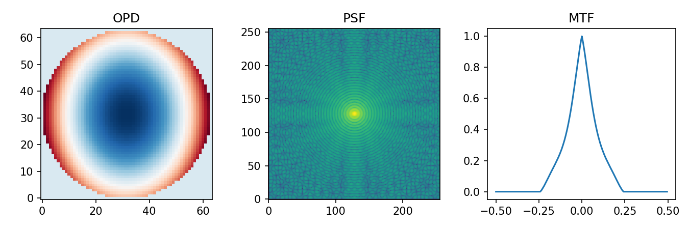
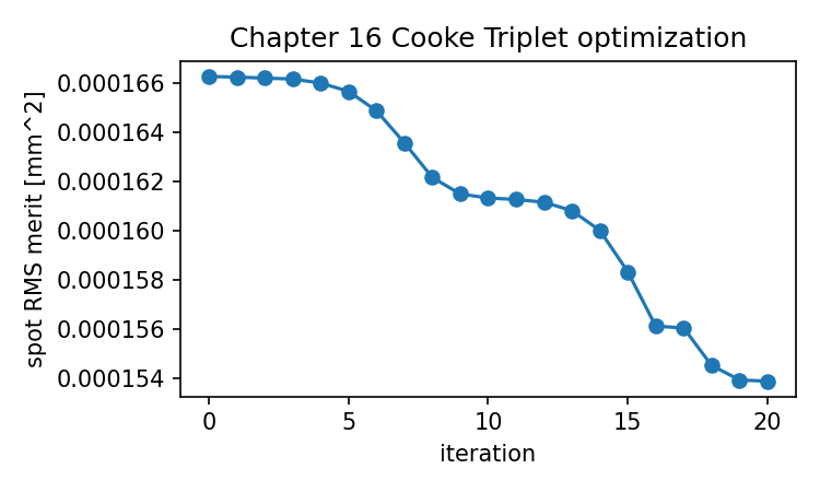
The iteration-level merit history is recorded in ../figures/chapter_16/cooke_optimization_history.csv.
Source and validation note
This chapter is the manuscript's full-chain validation anchor. The reported before/after merit values come from the pinned companion run with optiland==0.6.0; they should not be edited by hand. If the prescription, bounds, variables, fields, wavelengths, sampling, or Optiland version changes, rerun validation and replace both the chapter figures and the recorded merit history.