Computational Optics
Inspiration Overflow
This book explains how a lens prescription becomes ray data, wavefront error, a point spread function, and finally an MTF curve. The chapters use equations and executable Python examples together so that numerical conventions and assumptions remain visible.
How to use this book
Read the chapters in order if ray tracing or Fourier optics is new to you. Each chapter builds on definitions and conventions introduced earlier. Readers who already know geometrical optics may start at Chapter 10 for the wavefront-to-MTF computation.
The tested Python package, dependency lockfile, and reproduction commands are described in Companion Code.
Acknowledgements
Selected examples and validation tests use Optiland, an open-source optical design platform. We thank Kramer Harrison and the Optiland contributors for making it available under the MIT License. See the third-party notices.
License
The prose and figures are licensed under CC BY 4.0. Companion source code is licensed under the MIT License.
Chapter 1: Why MTF Does Not Come from a Software Button
A lens design program can make optics feel deceptively simple.
You build a lens. You enter a few radii, thicknesses, glasses, wavelengths, and field points. You click a button. A plot appears.
Maybe it is a spot diagram. Maybe it is a ray fan. Maybe it is a wavefront map. Or maybe it is the plot that many optical designers look at with a special mix of hope and dread: the MTF curve.
The curve looks authoritative. It has axes. It has sagittal and tangential lines. It has spatial frequency on one side and modulation on the other. If the lines stay high, the design looks promising. If they fall too early, something is wrong. The plot seems to speak in a clean engineering language:
This lens preserves contrast well.
This lens loses contrast at fine detail.
This field point is worse than the center.
This wavelength behaves differently.
This design is not ready yet.
That is all useful. But here is the problem.
Seeing an MTF curve is not the same as understanding where it came from.
This is not a complaint about optical design software. Good software hides labor, and in production work that is a gift. You do not want to manually compute every ray-surface intersection each time you adjust a radius. You do not want to write your own FFT every time you inspect diffraction performance. You want the tool to do those calculations quickly and reliably.
But learning is different from production.
For learning, the same convenience can become a wall. The software gives you the result, but the middle of the calculation disappears. You may learn to recognize a good MTF curve without knowing how that curve was built. You may know that PSF means point spread function, that OPD means optical path difference, and that MTF means modulation transfer function, but still not know how a lens prescription turns into those quantities.
That gap is the subject of this book.
We are going to open the box.
Not all at once. That would be unfair. The box contains geometry, vector math, ray tracing, first-order optics, wavefronts, sampling, Fourier transforms, normalization, units, and optimization. If we throw all of that at the reader in the first chapter, we have not taught anything. We have merely replaced one black box with another, more frightening one.
So we will begin with the map.
The curve that appears after you click the MTF button is not created by the button. It is the endpoint of a computation chain:
lens prescription
→ surfaces and materials
→ real ray tracing
→ paraxial reference
→ pupil sampling
→ optical path difference
→ pupil function
→ point spread function
→ optical transfer function
→ modulation transfer function
You do not need to understand every step yet. For now, just notice the shape of the chain. MTF sits near the end. It is not an isolated measurement floating above the optical system. It depends on the lens geometry, the glass, the wavelength, the aperture, the field point, the image plane, the wavefront error, and the numerical sampling method.
This is why a single MTF curve can be both powerful and dangerous.
Powerful, because it compresses many effects into one readable plot.
Dangerous, because the compression can make you forget the machinery underneath.
The curve is a consequence, not a starting point
Let us say we have a lens.
At the software level, the lens may appear as a table:
surface   radius      thickness     material     semi-diameter
0         infinity    infinity      air          —
1         50.0        5.0           N-BK7        10.0
2        -50.0        45.0          air          10.0
3         infinity    0.0           image        —
This is not just bookkeeping. It is the beginning of a computation.
Each row tells the program what kind of surface a ray may meet, where that surface is, how the ray should bend after reaching it, and where the next surface waits. A real optical design may contain many more surfaces, non-spherical shapes, apertures, solves, coatings, aspheric terms, multiple configurations, and multiple wavelengths. But the basic idea is the same:
A lens is not only a drawing. It is a structured set of inputs for calculation.
That is the first habit we need to build.
When you see a lens layout, ask: what data produced it?
When you see a ray trace, ask: how were the rays represented?
When you see a spot diagram, ask: where did those points come from?
When you see an MTF curve, ask: what chain of calculations created it?
This habit is more important than any single formula in the opening chapter. Formulae are easier to learn once you know where they belong.
A tiny preview of the computation chain
Before we touch a real optical system, let us look at a deliberately small piece of the chain.
In later chapters, we will compute wavefront error from traced rays. We will not cheat. We will build the ray model, intersect surfaces, refract directions, compare real rays to a reference, and construct OPD over the pupil.
For now, we will start halfway down the chain. Suppose we already have a pupil function. That means we know two things across the exit pupil:
- where light is allowed to pass;
- what phase delay the optical system has given to that light.
In scalar Fourier optics, a simplified pupil function can be written as:
P(x, y) = A(x, y) exp(i 2π W(x, y))
Here A(x, y) is the aperture amplitude mask. It may be 1 inside the pupil and 0 outside. W(x, y) is wavefront error measured in waves. The exponential turns wavefront error into optical phase.
Do not worry if this feels too fast. We will return to this carefully in the wavefront chapters. Right now, we only want to see that the PSF and MTF are not mystical objects. They can be computed.
Here is a minimal Python preview:
import numpy as np
import matplotlib.pyplot as plt

# A small square computational grid.
N = 256
u = np.linspace(-1.0, 1.0, N)
X, Y = np.meshgrid(u, u)
rho = np.sqrt(X**2 + Y**2)

# Circular pupil: light passes inside the unit circle.
aperture = rho <= 1.0

# A toy wavefront error in waves.
# This is not a full lens model yet. It is only a simple phase pattern.
defocus_waves = 0.5
W = defocus_waves * (2.0 * rho**2 - 1.0)

# Pupil function: amplitude mask times phase.
pupil = aperture * np.exp(1j * 2.0 * np.pi * W)

# PSF: squared magnitude of the Fourier transform of the pupil function.
amplitude = np.fft.fftshift(np.fft.fft2(np.fft.ifftshift(pupil)))
psf = np.abs(amplitude) ** 2
psf = psf / psf.sum()

# OTF: Fourier transform of the PSF.
otf = np.fft.fftshift(np.fft.fft2(np.fft.ifftshift(psf)))

# MTF: normalized magnitude of the OTF.
mtf = np.abs(otf)
mtf = mtf / mtf.max()

# A simple horizontal slice through the MTF.
center = N // 2
plt.plot(mtf[center, :])
plt.xlabel("sample index")
plt.ylabel("normalized modulation")
plt.title("A toy MTF slice from a toy pupil function")
plt.show()
This code is not yet a lens design program. It has no glass catalog, no curved surfaces, no Snell refraction, no image plane solve, no field angle, no physical frequency axis, and no careful sampling calibration. Good. It should not pretend to do more than it does.
But it shows something important.
The final line on the plot did not appear by magic. It came from data. The data came from a pupil. The pupil contained an aperture and a phase. The phase represented wavefront error. The PSF came from a Fourier transform of the pupil field. The OTF came from a Fourier transform of the PSF. The MTF came from the magnitude of the OTF.
Even in this toy example, the curve has ancestry.
That is the attitude we will keep throughout the book.
When a result appears, we will ask what produced it.
The software path and the learning path
A real optical design package does far more than the short script above.
It must know how to represent an optical system. It must trace rays through a sequence of surfaces. It must compute intersections between rays and surfaces. It must apply Snell’s law using local surface normals. It must handle stops, pupils, wavelengths, field points, and image surfaces. It must provide first-order quantities such as effective focal length and F-number. It must compute aberrations, wavefronts, PSF, MTF, and merit functions for optimization.
Open-source tools are useful here because they let us compare two levels of understanding:
minimum teaching code
real optical design library
The first level is our own small code. It is not complete, but it is transparent. It lets us see the skeleton of the algorithm.
The second level is a real library. It handles more cases, uses better internal organization, and connects the calculation to practical optical design workflows.
In this book, Optiland will serve as our main open-source reference implementation. Its current documentation describes it as a Python-based open-source framework for optical design, analysis, and optimization, with support for paraxial, real, and polarization-aware ray tracing, wavefront analysis, PSF/MTF analysis, scattering, optimization, visualization, and differentiable machine-learning workflows. The same documentation also notes that the project is under active development, which is exactly why we will keep the principles separate from any one version of the API. (optiland.readthedocs.io)
That last sentence matters.
Optiland is not the hero of this book.
The computation chain is the hero.
Optiland is valuable here because it gives us inspectable, executable machinery. We are not memorizing one library’s API; we are learning the calculations any serious optical design tool must perform in some form.
For example, current Optiland examples show compact calls for loading sample lenses, drawing layouts, tracing rays, creating spot diagrams, and computing PSF and MTF. A small preview may look like this: (optiland.readthedocs.io)
from optiland.samples.objectives import CookeTriplet
from optiland.analysis import SpotDiagram
from optiland.psf import FFTPSF
from optiland.mtf import FFTMTF

lens = CookeTriplet()

# Draw the optical layout.
lens.draw()

# A geometric ray-based analysis.
spot = SpotDiagram(lens)
spot.view()

# A diffraction-based PSF calculation.
psf = FFTPSF(lens, field=(0, 0), wavelength="primary")
psf.view(projection="2d", num_points=256)

# An MTF calculation.
mtf = FFTMTF(lens)
mtf.view()
This is the kind of code that makes modern optical computation feel approachable. But we should be careful. A short library call can become a new black box if we stop there.
So we will usually read such code in two ways.
The first reading is practical:
Good, this is how I ask the library for a PSF or MTF.
The second reading is computational:
What must the library already know in order to answer?
For FFTPSF(lens, field=(0, 0), wavelength="primary") to work, the program must have access to a defined optical system, a field point, a wavelength, an aperture, a method for constructing wavefront information, and a sampling strategy. For FFTMTF(lens) to work, it must eventually produce or use information equivalent to a PSF or OTF, then normalize and display contrast response against spatial frequency.
The call is short because the library has already organized the work.
The work is still there.
What MTF actually says
Let us pause and make the physical meaning less abstract.
A perfect black-and-white bar pattern has strong contrast. The dark bars are dark, the bright bars are bright. If an optical system images that pattern poorly, the bright bars bleed into the dark bars. Fine detail becomes gray mush. The modulation has dropped.
MTF measures how much contrast survives at different spatial frequencies.
Low spatial frequency means broad detail: large letters, thick bars, slow changes across the image.
High spatial frequency means fine detail: thin lines, small texture, sharp edges.
An optical system may preserve low-frequency contrast well while losing high-frequency contrast. This is why an image can look generally clear but still lack fine detail. It is also why a single “sharp/not sharp” judgment is too crude for optical design.
MTF gives us a more structured question:
At this field point,
for this wavelength or wavelength weighting,
in this direction,
at this spatial frequency,
how much modulation remains?
That question is already full of conditions. There is no free-floating MTF. There is always MTF for a system, at a field, under a wavelength condition, with a sampling and calculation method.
This is one reason beginners get confused. The plot looks like one object, but it has many hidden inputs.
Here we can slow down.
You do not need to memorize every condition yet. Just remember that when you see an MTF curve, you are not looking at “the quality of the lens” in some absolute sense. You are looking at one computed view of the lens under defined assumptions.
That makes the curve more useful, not less. It means we can ask better questions.
If the MTF drops off-axis, is the culprit astigmatism? Coma? Field curvature? A sampling issue? Defocus? A bad image plane location? Wavelength weighting? A real design limitation?
The curve alone cannot answer all of that. But once we understand the chain that produced it, we can trace the problem backward.
The first black box: the lens prescription
Every calculation begins with inputs. In optical design, the most important input is the prescription.
A prescription is the optical system written as data. It tells us the sequence of surfaces that light encounters. A simple surface entry may include:
radius of curvature
thickness to the next surface
material after the surface
semi-aperture
conic constant
surface type
In a lens drawing, you see curved glass.
In a prescription, the computer sees instructions.
A spherical surface with radius R is not just a pretty boundary. It is a geometric object. When a ray approaches it, the program has to solve a ray-sphere intersection problem. After the intersection point is found, the program has to compute the surface normal. Then it has to use the refractive indices on both sides of the surface to compute the outgoing direction.
That means the MTF curve at the end depends on many earlier decisions that sound humble:
How did we store the surface?
How did we compute the intersection?
Which refractive index did we use at this wavelength?
Where is the stop?
Which rays were sampled?
Where is the image surface?
This is why Chapter 2 will not begin with image quality. It will begin with the prescription.
We will take the lens out of the drawing and write it as a data structure. That may sound less glamorous than MTF, but it is the correct beginning. If the optical system is not represented clearly, every later calculation becomes foggy.
The second black box: ray tracing
After the lens is represented, the program traces rays.
A ray can be written as:
r(t) = r0 + t d
Here r0 is the starting point, d is the direction vector, and t is the distance parameter along the ray. This small equation is one of the quiet workhorses of optical computation.
To trace a ray through a lens, the program repeatedly asks:
Where does this ray hit the next surface?
What is the normal at that point?
What is the refractive index before and after the surface?
What direction does Snell's law give after refraction?
Does the ray pass through the aperture?
Where does it land on the image surface?
This is not conceptually mystical. It is a sequence of geometry and vector operations.
But it is easy to skip in textbooks because the algebra is not always elegant. It is also easy to hide in software because users usually want the output, not the intersection routine. As a result, many learners jump from “Snell’s law exists” to “the software traces rays,” with the actual calculation missing in between.
We will not skip it.
Chapters 4, 5, and 6 are the root system of this book. We will define a ray, compute where it hits a plane or sphere, and calculate the refracted direction. These chapters may feel modest compared with PSF and MTF, but they are where the black box first opens.
If ray tracing is unclear, everything later becomes a ritual.
If ray tracing is clear, spot diagrams, ray fans, and wavefronts become much less mysterious.
The third black box: from rays to wavefront
A spot diagram can be built from ray intersections. Trace many rays through the pupil, let them hit the image surface, and plot the points. That already tells us a lot about geometric blur.
But PSF and diffraction MTF require another representation.
They need wavefront information.
This is the bridge that many learners feel but cannot name. Geometric optics talks about rays. Fourier optics talks about complex fields, pupil functions, diffraction patterns, and transforms. A practical optical design program must connect these worlds.
That connection often runs through optical path length and optical path difference.
Roughly speaking, optical path length measures phase travel through media with refractive index. OPD compares the actual optical path to a reference path. Once OPD is known across the pupil, it can be translated into phase. Once phase is known across the pupil, we can form the pupil function. Once we have the pupil function, we can compute the PSF.
That is the moment when the toy code from earlier starts to make sense.
The toy code began with a pupil function. In the full book, we will earn that pupil function from the optical system.
The chain will become:
trace rays through the lens
→ compute optical path differences over the pupil
→ convert OPD into phase
→ build the pupil function
→ Fourier transform to obtain the PSF
At first glance, this looks like a lot. It is a lot. But the difficulty is not that any single step is magical. The difficulty is that the steps belong to different mental toolkits.
Geometry gives us rays.
Physical optics gives us phase.
Numerical computation gives us arrays and FFTs.
Optical engineering gives us interpretation.
This book is about stitching those toolkits together.
The fourth black box: from PSF to MTF
Once we have the PSF, MTF is close, but still not automatic in the human sense.
The PSF tells us how a point object spreads in the image. A perfect point would remain a point. A real optical system spreads it because of diffraction, aberration, defocus, sampling, and other effects.
The optical transfer function, or OTF, describes how the system transfers spatial frequency content. In simplified computational terms:
OTF = Fourier transform of PSF
MTF = magnitude of OTF
Usually we normalize the MTF so that the zero-frequency value is 1. That gives us a curve where modulation begins at 1 and generally decreases as spatial frequency increases.
This compact relationship is one reason MTF feels simple once it is presented. But the simplicity is deceptive. The PSF already contains the consequences of everything before it. The MTF inherits all of that.
A bad MTF curve is not merely “bad MTF.”
It may be telling you about aberrations. Or focus. Or field position. Or aperture. Or wavelength. Or sampling. Or an error in how the calculation was set up.
That is why this book does not treat MTF as a standalone chapter at the beginning. We start with the question, but we do not pretend the answer is immediate.
We will reach MTF properly in Chapter 13. By then, the curve should no longer feel like a software oracle. It should feel like the final plot of a calculation you can inspect.
What this book will do differently
Many optical books are excellent at explaining principles. Many software manuals are excellent at explaining commands. Both are valuable. But there is a gap between them.
The gap looks like this:
I know the formula.
I know the software button.
But I do not know the computation that connects them.
This book lives in that gap.
For each major idea, we will use three layers.
First, the optical principle:
What physical or geometric problem are we solving?
Second, the computational form:
What variables, equations, arrays, and algorithms represent that problem?
Third, executable code:
Can we write a small version ourselves, then compare it with a real tool?
The small version is important. It prevents us from using Optiland, or any library, as a replacement black box.
The real-tool comparison is also important. It prevents us from writing toy code that never touches practical optical design.
You can think of the book as two rails:
Rail A: minimal Python implementations
Rail B: Optiland reference workflows
Rail A teaches the bones.
Rail B shows how the bones live inside a more complete body.
We will move between them carefully.
A warning about code examples
Optical code is sensitive to convention.
Units matter. Sign conventions matter. Surface indexing matters. Wavelength units matter. Coordinate systems matter. FFT normalization matters. Whether a field is specified by angle or object height matters. Whether frequency is cycles per millimeter or normalized sample index matters.
This means code examples in optics should be read with more care than ordinary programming snippets.
When we write a few lines of NumPy, we are often choosing a convention silently. When we call a library, the library has already chosen many conventions for us. A large part of learning computational optics is learning to ask:
What are the units?
What is being normalized?
Where is the origin?
Which plane are we in?
Which wavelength is primary?
Which field point is this?
What does the plotted axis actually mean?
This may sound fussy. It is not. These questions are the difference between understanding a plot and merely admiring it.
Later, Chapter 14 will be devoted to exactly this kind of trouble: sampling, normalization, FFT shifts, frequency axes, and unit conversion. That chapter may save you many hours of confusion. It is not glamorous, but it is kind.
What you should be able to do after this chapter
After this chapter, you should not yet be able to implement a complete MTF calculation from a real lens prescription. That would be too much to ask.
But you should be able to say something more precise than:
The software calculates MTF.
You should be able to say:
The MTF curve is the endpoint of a chain. The system begins as a lens prescription. Rays are traced through surfaces and materials. The program builds geometric and wavefront information at a field and wavelength. The pupil function leads to the PSF. The PSF leads to the OTF. The magnitude of the OTF gives the MTF.
That is already a large step.
You have moved from result-watching to process-thinking.
This shift changes how you read every optical plot.
A spot diagram is no longer just a scatter plot. It is the record of many traced rays landing on an image plane.
A ray fan is no longer just a diagnostic curve. It is a structured view of transverse ray error across the pupil.
An OPD map is no longer just colored decoration. It is a bridge between ray geometry and wave phase.
A PSF is no longer just a blur image. It is the intensity distribution produced by the pupil field.
An MTF curve is no longer just a button output. It is the frequency-domain summary of image contrast transfer.
This is the whole direction of the book.
We are not trying to make optical design look easy. That would be dishonest. Optical design is demanding.
But demanding is not the same as mysterious.
Much of the mystery comes from missing steps. Once the steps are visible, the subject becomes more teachable. Still difficult, yes. But no longer sealed away.
The road ahead
In the next chapter, we will go back to the beginning of the chain.
Before we trace rays, before we compute wavefronts, before we talk about PSF or MTF again, we need to answer a plain question:
What exactly is a lens prescription?
Not as a PDF table.
Not as a drawing.
As data.
We will take the optical system apart into radius, thickness, material, aperture, wavelength, and field. Then we will write a small Python representation of a simple lens. After that, when a ray moves through the system, it will no longer be moving through a vague diagram. It will be moving through data we can inspect.
That is where computational optics begins.
Not with the MTF button.
With the inputs that make the button possible.
Generated validation figure
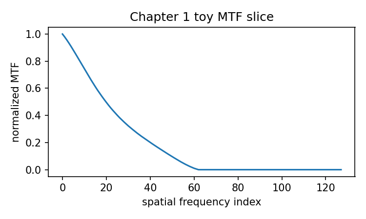
Source and validation note
Software-facing statements in this chapter are version-bounded. The companion project is pinned to optiland==0.6.0; PyPI records that release separately from the public Read the Docs pages, which may update independently. The main claim of this chapter does not depend on one Optiland API call. It depends on the stable computation chain: prescription, tracing, wavefront or pupil representation, PSF, OTF, and MTF.
Chapter 2: What a Lens Prescription Really Is
A lens drawing is easy to like.
You see curved pieces of glass. You see air gaps. You see a stop. You may see rays bending through the system and meeting near an image plane. A drawing gives your eyes something to hold onto.
But a drawing is not what the optical software calculates from.
The software needs a prescription.
At first, a lens prescription looks disappointingly plain. It is usually a table: surface number, radius, thickness, material, aperture, maybe conic constant, maybe aspheric coefficients, maybe comments. Compared with a ray-traced layout or an MTF plot, it looks almost bureaucratic.
That plainness is the point.
A lens prescription is the optical system written as data.
Once the system is written as data, a program can do something with it. It can compute surface positions. It can ask where a ray intersects the next surface. It can look up refractive index at a wavelength. It can decide whether a ray is blocked by an aperture. It can trace many rays to an image plane. Later, it can build spot diagrams, wavefront maps, PSF images, and MTF curves.
So before we trace rays, before we calculate OPD, before we touch Fourier transforms, we need to learn a modest but crucial skill:
We need to read a lens prescription as a computational object.
This chapter is about that object.
Not about a beautiful optical layout. Not about final image quality. Just the data structure that makes all later calculations possible.
That may sound like a small step. It is not. If the prescription is unclear, everything downstream becomes unclear. A wrong surface radius, a misunderstood thickness, or a misplaced material assignment can quietly poison the entire calculation chain.
Here we can be explicit. We are not memorizing a professional lens design table; we are turning a piece of glass into data a Python program can use.
A prescription is a sequence
Most introductory optical drawings make a lens look like an object in space. A prescription makes it look like a sequence.
Light travels through one surface, then the next, then the next. In a sequential optical system, surfaces are ordered along the optical path. The program does not first see “a lens” in the human sense. It sees something more like this:
surface 0 → surface 1 → surface 2 → surface 3 → ...
Each surface tells the program:
Where am I?
What shape am I?
What medium comes after me?
How far is the next surface?
How large is the usable aperture here?
For a simple singlet lens, a minimal table might look like this:
surface   radius      thickness     material     semi-diameter     note
0         infinity    infinity      air          —                 object
1         +50.0       5.0           N-BK7        10.0              front lens surface
2         -50.0       45.0          air          10.0              back lens surface
3         infinity    0.0           air          —                 image plane
This is already enough to teach several important conventions.
The first row is often the object surface. If the object is at infinity, the radius and thickness may be represented as infinity. This does not mean the software is trying to draw an infinitely large surface. It means the incoming rays are treated according to an object-at-infinity convention.
Surface 1 is the first physical glass surface. Its radius is positive in this example. It has a thickness of 5.0, which means the distance from surface 1 to surface 2 along the optical axis is 5.0 units. If we use millimeters, then this is 5.0 mm.
The material listed at surface 1 is N-BK7. In the usual sequential prescription convention, this means the medium after surface 1 is N-BK7. In other words, once a ray crosses surface 1, it travels through N-BK7 until it reaches surface 2.
Surface 2 has material air, which means after crossing surface 2, the ray leaves the glass and travels in air toward the image plane.
Surface 3 is the image plane. It is still treated as a surface in the sequence, even though it may not be a physical piece of glass.
This is the first useful mental shift:
The image plane is not just “where the drawing ends.” In computation, it is another target surface where ray positions can be evaluated.
That is how a spot diagram eventually becomes possible. The program traces rays through the earlier surfaces, then asks where they land on the image surface.
The main columns
Let us unpack the common columns one by one.
A basic lens prescription often includes these fields:
radius
thickness
material
semi-diameter
conic constant
surface type
Professional software may include many more: coating, aperture type, solve type, pickup, coordinate break, aspheric coefficients, diffractive terms, thermal model, tolerance data, and so on. We do not need all of that yet.
For now, the six fields above are enough to build the first data structure.
Radius: the surface curvature in human form
The radius tells us how curved a surface is.
For a spherical surface, the radius is the radius of the sphere from which the surface is cut. A large radius means a gentle surface. An infinite radius means a plane. A small radius means a stronger curve.
In many optical prescriptions, the radius is signed. The sign convention depends on the coordinate system, and different tools may define signs carefully in their own way. In this book, we will use the common sequential optics intuition: light travels roughly in the positive z direction, and the sign of the radius tells us where the center of curvature lies relative to the surface vertex.
For now, do not let the sign convention become a monster under the bed. We will make it explicit in code whenever it matters.
A radius is often converted into curvature:
c = 1 / R
If R is infinite, the curvature is zero. That is exactly what we want for a plane surface.
This small conversion is common because many equations are cleaner when written in terms of curvature c rather than radius R.
In code, we should handle infinity gently. A plane surface should not cause a divide-by-infinity surprise or a special-case disaster. We can write a helper function:
import math

def curvature_from_radius(radius):
    """Return curvature c = 1/R, with planes represented by c = 0."""
    if math.isinf(radius):
        return 0.0
    return 1.0 / radius

print(curvature_from_radius(50.0))        # 0.02
print(curvature_from_radius(float("inf"))) # 0.0
This is not glamorous code. But it is exactly the kind of small convention that keeps an optical program sane.
Thickness: distance to the next surface
Thickness is one of the most easily misunderstood columns.
In a sequential prescription, thickness usually means:
the axial distance from this surface to the next surface.
It does not mean “the thickness of this surface.” A mathematical surface has no thickness. It is a boundary. The thickness column tells us how far to move before reaching the next boundary.
For a physical lens element, the thickness after the first surface is often the glass center thickness. For an air gap, the thickness after the second surface may be the distance through air to the next optical element or image plane.
In our simple singlet:
surface 1 thickness = 5.0
means the axial distance from the front glass surface to the back glass surface is 5.0 mm.
surface 2 thickness = 45.0
means the axial distance from the back glass surface to the image plane is 45.0 mm.
This convention matters because it defines the global positions of the surfaces.
If surface 1 is at z = 0, then surface 2 is at z = 5, and surface 3 is at z = 50.
That is already a little optical system in coordinates.
Let us compute those positions.
from dataclasses import dataclass
from typing import Optional
import math

@dataclass
class Surface:
    radius: float
    thickness: float
    material_after: str = "air"
    semi_diameter: Optional[float] = None
    conic: float = 0.0
    comment: str = ""

def surface_vertices(surfaces):
    """Return the z-coordinate of each surface vertex."""
    z = 0.0
    vertices = []

    for s in surfaces:
        vertices.append(z)

        # The last image surface may have thickness 0.
        # An infinite object thickness should not move our finite drawing origin.
        if not math.isinf(s.thickness):
            z += s.thickness

    return vertices

surfaces = [
    Surface(radius=float("inf"), thickness=float("inf"), comment="object at infinity"),
    Surface(radius=+50.0, thickness=5.0, material_after="N-BK7",
            semi_diameter=10.0, comment="front lens surface"),
    Surface(radius=-50.0, thickness=45.0, material_after="air",
            semi_diameter=10.0, comment="back lens surface"),
    Surface(radius=float("inf"), thickness=0.0, material_after="air",
            comment="image plane"),
]

# For a simple finite layout, we usually start drawing at the first physical surface.
finite_surfaces = surfaces[1:]
for i, (s, z) in enumerate(zip(finite_surfaces, surface_vertices(finite_surfaces)), start=1):
    print(i, z, s.comment)
This prints surface positions for the finite part of the system. We skipped the object-at-infinity row when computing drawing coordinates, because it is a boundary condition, not a finite physical surface.
Already, the prescription has become something a program can inspect.
Material: the medium after the surface
The material column tells us what medium the ray enters after crossing a surface.
This is worth repeating because it is a common source of mistakes:
In a sequential prescription, material usually belongs to the space after the surface, not before it.
For surface 1 in the singlet, the material after the surface is glass. For surface 2, the material after the surface is air.
That means each surface interaction needs two refractive indices:
n_before → n_after
At surface 1, for a ray entering the lens:
air → N-BK7
At surface 2:
N-BK7 → air
We will not calculate refraction in this chapter. That comes later. But the prescription already contains the information needed for it.
For now, we can add a very small material model. It will not handle real dispersion yet. Chapter 3 will handle wavelength and refractive index more carefully. Here, we only want the data structure to know that different media exist.
SIMPLE_INDEX = {
    "air": 1.0,
    "N-BK7": 1.5168,  # approximate value near the yellow helium d-line
}

def refractive_index(material_name, wavelength_um=0.5876):
    """A placeholder material model.

    Chapter 3 will replace this with wavelength-dependent glass behavior.
    """
    try:
        return SIMPLE_INDEX[material_name]
    except KeyError:
        raise ValueError(f"Unknown material: {material_name}")

def media_before_after(surfaces, surface_index, starting_material="air"):
    """Return material before and after a surface in a sequential system."""
    if surface_index == 0:
        before = starting_material
    else:
        before = surfaces[surface_index - 1].material_after

    after = surfaces[surface_index].material_after
    return before, after

for i, s in enumerate(finite_surfaces):
    before, after = media_before_after(finite_surfaces, i)
    print(f"Surface {i+1}: {before} -> {after}")
A real optical library will use a glass catalog and compute refractive index as a function of wavelength. Our placeholder is deliberately simple. It is a signpost, not a finished material engine.
The important point is structural:
Refraction later depends on material transitions that are already encoded in the prescription.
Semi-diameter: the usable size of the surface
The semi-diameter is the usable radius of the surface aperture. If the semi-diameter is 10 mm, the clear circular region has a diameter of 20 mm.
It is tempting to treat semi-diameter as merely a drawing parameter. Do not do that. It is also a ray-blocking parameter.
A ray may geometrically intersect a spherical surface, but if the intersection point lies outside the usable semi-diameter, the ray should be considered blocked or invalid for that surface.
In a simple circular aperture check:
sqrt(x² + y²) <= semi_diameter
or, more efficiently:
x² + y² <= semi_diameter²
In code:
def inside_clear_aperture(x, y, semi_diameter):
    if semi_diameter is None:
        return True
    return x*x + y*y <= semi_diameter*semi_diameter

print(inside_clear_aperture(3.0, 4.0, 5.0))  # True
print(inside_clear_aperture(6.0, 0.0, 5.0))  # False
This tiny check will matter later when we trace a bundle of rays. Some rays will pass through the clear aperture. Some will be clipped. The final spot diagram, illumination pattern, PSF, and MTF can all be affected by aperture definitions.
Again, the later plot begins here, in the plain table.
Stop surface: the aperture that controls the beam
Not every semi-diameter is the aperture stop.
Every surface may have a clear aperture, but the aperture stop is the element that limits the cone of rays through the system. In many optical systems, the stop may be a physical diaphragm. In simple examples, a lens surface itself may be marked as the stop.
A prescription often marks one surface as the stop:
surface 1: is_stop = True
This is not just a note for drawing. The stop helps determine entrance pupil, exit pupil, ray sampling, F-number, and which rays are considered part of the imaging bundle.
For now, we can add an is_stop field to our Surface class.
@dataclass
class Surface:
    radius: float
    thickness: float
    material_after: str = "air"
    semi_diameter: Optional[float] = None
    conic: float = 0.0
    is_stop: bool = False
    comment: str = ""
This does not yet calculate pupils. It simply records the information. Later chapters will use it.
This is a recurring pattern in computational optics:
record the optical data first
then write algorithms that consume that data
If the data structure is vague, the algorithms become a mess.
Conic constant: the first step beyond spheres
A sphere is not the only useful optical surface.
Many lenses use conic or aspheric surfaces to control aberrations. The conic constant describes how the surface deviates from a sphere into shapes such as paraboloids, ellipsoids, or hyperboloids.
The sag of a rotationally symmetric conic surface can be written as:
z(r) = (c r²) / (1 + sqrt(1 - (1 + k)c²r²))
where:
r = sqrt(x² + y²)
c = 1 / R
k = conic constant
For a sphere, k = 0.
At this point, you do not need to memorize the sag equation. Just see what it does. It turns a surface prescription into a height function. Given a radial distance r from the optical axis, it tells us the z sag of the surface relative to its vertex.
This matters because ray-surface intersection eventually asks:
Where does the ray meet this actual surface shape?
For this chapter, we will only evaluate the sag. We will not solve full ray-asphere intersections yet.
import numpy as np

def conic_sag(r, radius, conic=0.0):
    """Sag z(r) for a rotationally symmetric conic surface."""
    if math.isinf(radius):
        return np.zeros_like(r, dtype=float)

    c = 1.0 / radius
    inside = 1.0 - (1.0 + conic) * (c * r)**2

    # Numerical guard for values very close to zero.
    inside = np.maximum(inside, 0.0)

    return (c * r**2) / (1.0 + np.sqrt(inside))

r = np.linspace(0.0, 10.0, 6)
print(conic_sag(r, radius=50.0, conic=0.0))
The output values are small near the axis and grow toward the edge. That is the surface becoming curved.
If you want to visualize it:
import matplotlib.pyplot as plt

r = np.linspace(0.0, 10.0, 200)

plt.plot(r, conic_sag(r, radius=50.0, conic=0.0), label="sphere, R=50")
plt.plot(r, conic_sag(r, radius=50.0, conic=-1.0), label="paraboloid-like, k=-1")
plt.xlabel("radial coordinate r [mm]")
plt.ylabel("sag z [mm]")
plt.title("Conic sag profiles")
plt.legend()
plt.show()
This is a quiet but important moment. A row in a table has become a mathematical surface. The surface has become a function. A function can be evaluated. Later, a ray can intersect it.
That is how the black box starts opening.
Surface type: plane, sphere, conic, asphere
The surface type tells the program what geometry model to use.
A minimal program may support only:
plane
sphere
A practical design tool may support:
standard spherical surface
conic surface
even asphere
odd asphere
toroidal surface
freeform surface
coordinate break
diffractive surface
mirror
image surface
Each type implies different geometry and different intersection logic.
This is why a surface data structure should not only store numbers. It should also store what those numbers mean.
For our teaching code, we can start with:
@dataclass
class Surface:
    radius: float
    thickness: float
    material_after: str = "air"
    semi_diameter: Optional[float] = None
    conic: float = 0.0
    is_stop: bool = False
    surface_type: str = "spherical"
    comment: str = ""
If surface_type is "spherical" and the radius is infinite, we can treat it as a plane. If it is "image", we know it is the final evaluation plane. A richer program would use separate classes for different surface types. For teaching, a field is enough.
Chapter 2 is not about perfect optical software architecture. It is about making the computational meaning visible.
A complete minimal prescription object
Now we can gather the pieces.
A lens system is more than a list of surfaces. It also has system-level settings:
aperture definition
field points
wavelengths
units
The surfaces describe the sequential geometry. The system settings describe how we illuminate and evaluate the system.
Let us write a small LensSystem.
from dataclasses import dataclass, field
from typing import List, Optional
import math

@dataclass
class Surface:
    radius: float
    thickness: float
    material_after: str = "air"
    semi_diameter: Optional[float] = None
    conic: float = 0.0
    is_stop: bool = False
    surface_type: str = "spherical"
    comment: str = ""

    @property
    def curvature(self):
        if math.isinf(self.radius):
            return 0.0
        return 1.0 / self.radius

@dataclass
class LensSystem:
    surfaces: List[Surface] = field(default_factory=list)
    aperture_type: str = "EPD"
    aperture_value: float = 10.0
    field_type: str = "angle"
    fields: List[float] = field(default_factory=lambda: [0.0])
    wavelengths_um: List[float] = field(default_factory=lambda: [0.5876])
    units: str = "mm"

    def add_surface(self, surface: Surface):
        self.surfaces.append(surface)

    def finite_vertices(self):
        """Return z positions for finite surfaces after skipping object at infinity."""
        finite = self.surfaces

        if finite and math.isinf(finite[0].thickness):
            finite = finite[1:]

        z = 0.0
        vertices = []
        for s in finite:
            vertices.append(z)
            if not math.isinf(s.thickness):
                z += s.thickness
        return vertices

    def print_prescription(self):
        print(" idx | radius | curvature | thickness | material | semi-dia | stop | comment")
        print("-----+--------+-----------+-----------+----------+----------+------+---------")
        for i, s in enumerate(self.surfaces):
            sd = "" if s.semi_diameter is None else f"{s.semi_diameter:.3g}"
            print(
                f"{i:>4} | "
                f"{s.radius:>7g} | "
                f"{s.curvature:>9.4g} | "
                f"{s.thickness:>9g} | "
                f"{s.material_after:>8} | "
                f"{sd:>8} | "
                f"{str(s.is_stop):>4} | "
                f"{s.comment}"
            )
Now define our singlet:
lens = LensSystem(aperture_type="EPD", aperture_value=10.0)

lens.add_surface(Surface(
    radius=float("inf"),
    thickness=float("inf"),
    material_after="air",
    surface_type="object",
    comment="object at infinity"
))

lens.add_surface(Surface(
    radius=+50.0,
    thickness=5.0,
    material_after="N-BK7",
    semi_diameter=10.0,
    is_stop=True,
    comment="front lens surface"
))

lens.add_surface(Surface(
    radius=-50.0,
    thickness=45.0,
    material_after="air",
    semi_diameter=10.0,
    comment="back lens surface"
))

lens.add_surface(Surface(
    radius=float("inf"),
    thickness=0.0,
    material_after="air",
    surface_type="image",
    comment="image plane"
))

lens.print_prescription()

print("\nFinite surface vertex positions:")
for z in lens.finite_vertices():
    print(z)
This is not yet ray tracing. It is something more basic:
It is a computable description of the optical system.
That description now contains the minimum information needed for later algorithms.
Chapter 3 will improve the material model. Chapter 4 will define rays. Chapter 5 will use the surface geometry to calculate intersections. Chapter 6 will use material transitions to calculate refraction.
The chain is already visible.
Why object and image are also surfaces
Beginners often want to remove the object and image rows because they are not physical lens elements.
Please resist that urge.
In sequential optics, object and image surfaces are useful because they make the system uniform. They let the program treat the optical path as a sequence with a beginning and an end.
The object surface defines how rays start. If the object is at infinity, rays from an on-axis field point enter parallel to the optical axis. If the object is finite, rays may start from a finite object height.
The image surface defines where rays are evaluated. A spot diagram is built from ray coordinates at the image surface. A focus shift can be represented by moving the image surface. Optimization may vary the final thickness to improve image quality.
So even when these rows look artificial, they serve a computational purpose.
They answer two questions:
How do rays enter the system?
Where do we measure their result?
Without those two answers, the lens is just glass floating in space.
The prescription is not the picture
Let us make this distinction very clear.
A prescription table can produce a drawing, but it is not the same thing as a drawing.
The drawing is a visualization derived from the data. The prescription is the data.
This matters because a drawing may hide details. It may not show exact radii. It may exaggerate shapes for readability. It may omit aperture limits or conic terms. It may not show wavelength, field, or material dispersion. A prescription, if complete, stores the details needed for computation.
In code, a drawing call should come after the data has been built:
prescription data → layout drawing
not the other way around.
This may feel obvious, but it saves confusion later. When software draws a lens, the drawing is not the source of truth. The source of truth is the optical model behind the drawing.
Optiland version of the same idea
Our small Python structure is useful because it exposes the skeleton. A real optical design library needs a more complete model.
Optiland’s documentation presents the Optic class as the primary interface for defining optical systems and describes surfaces as building blocks for optical elements. Its beginner example constructs a singlet by adding surfaces, setting an aperture, adding a field, adding a wavelength, drawing the system, and tracing rays. (Optiland) The current cheat sheet shows the same surface-by-surface pattern: create an optic.Optic(), add object, lens, and image surfaces, set entrance pupil diameter, field type, and wavelength. (Optiland)
A compact Optiland version of our singlet looks like this:
from optiland import optic

lens = optic.Optic()

# Object surface: object at infinity.
lens.surfaces.add(
    index=0,
    radius=float("inf"),
    thickness=float("inf")
)

# Front surface of the singlet.
# The material is the medium after this surface.
lens.surfaces.add(
    index=1,
    radius=50.0,
    thickness=5.0,
    material="N-BK7",
    is_stop=True
)

# Back surface of the singlet.
# After this surface, rays travel in air.
lens.surfaces.add(
    index=2,
    radius=-50.0,
    thickness=45.0
)

# Image surface.
lens.surfaces.add(index=3)

# System-level settings.
lens.set_aperture(aperture_type="EPD", value=10.0)
lens.fields.set_type("angle")
lens.fields.add(y=0.0)
lens.wavelengths.add(value=0.5876, is_primary=True)

lens.draw(num_rays=5)
Do not rush past this code.
It is doing the same conceptual work as our teaching structure. It creates a sequential optical system. It adds surfaces. It assigns material after a surface. It identifies a stop. It sets aperture, field, and wavelength. Then it draws the system.
The Optiland code is shorter because the library already knows how to organize optical objects. Our teaching code is more explicit because we want to see the bones.
Both are useful.
If we only use the teaching code, we risk building a toy world that never touches real optical software practice.
If we only use Optiland calls, we risk replacing one black box with another.
So we will keep both rails.
What the Optiland call hides on purpose
When we write:
lens.surfaces.add(index=1, radius=50.0, thickness=5.0, material="N-BK7")
a lot is being delegated.
The library must store the surface. It must decide how to represent the geometry. It must connect this surface to the next one. It must know how to look up the material later. It must participate in drawing, ray tracing, paraxial analysis, and optimization.
That is good software design. A library should not make the user manually wire every internal detail.
But as learners, we should still ask:
What does this one line imply?
It implies a surface vertex. It implies curvature. It implies a medium transition. It implies a distance to the next surface. It implies future ray-surface intersection. It implies future refraction.
A short API call is not a small optical event. It is a compact representation of many later computations.
That is the exact habit we are trying to build.
A small prescription reader
Professional lens files have their own formats. We will not build a full file parser here. But it is useful to see how close a prescription table is to code.
Suppose we write the surface data as a list of dictionaries:
raw_prescription = [
    {
        "radius": float("inf"),
        "thickness": float("inf"),
        "material_after": "air",
        "surface_type": "object",
        "comment": "object at infinity",
    },
    {
        "radius": 50.0,
        "thickness": 5.0,
        "material_after": "N-BK7",
        "semi_diameter": 10.0,
        "is_stop": True,
        "comment": "front lens surface",
    },
    {
        "radius": -50.0,
        "thickness": 45.0,
        "material_after": "air",
        "semi_diameter": 10.0,
        "comment": "back lens surface",
    },
    {
        "radius": float("inf"),
        "thickness": 0.0,
        "material_after": "air",
        "surface_type": "image",
        "comment": "image plane",
    },
]
Then build a LensSystem:
def build_lens_from_dicts(rows):
    lens = LensSystem()
    for row in rows:
        lens.add_surface(Surface(
            radius=row["radius"],
            thickness=row["thickness"],
            material_after=row.get("material_after", "air"),
            semi_diameter=row.get("semi_diameter"),
            conic=row.get("conic", 0.0),
            is_stop=row.get("is_stop", False),
            surface_type=row.get("surface_type", "spherical"),
            comment=row.get("comment", ""),
        ))
    return lens

lens = build_lens_from_dicts(raw_prescription)
lens.print_prescription()
This is simple, but the meaning is large.
A lens prescription can be stored, loaded, transformed, checked, drawn, traced, optimized, and compared.
That is why optical design software begins with tables. Tables are not an old-fashioned interface choice. They are a natural way to expose a sequential model.
Sanity checks before tracing rays
Before a program traces even one ray, it should check the prescription for obvious problems.
For example:
Is there at least one surface?
Is there an image surface?
Is there a stop or aperture definition?
Are finite thicknesses non-negative?
Are materials known?
Are semi-diameters positive when present?
Let us write a few simple checks.
def validate_lens(lens):
    errors = []

    if not lens.surfaces:
        errors.append("Lens has no surfaces.")

    if lens.surfaces and lens.surfaces[-1].surface_type != "image":
        errors.append("Last surface is not marked as an image surface.")

    if not any(s.is_stop for s in lens.surfaces):
        errors.append("No stop surface is marked.")

    for i, s in enumerate(lens.surfaces):
        if not math.isinf(s.thickness) and s.thickness < 0:
            errors.append(f"Surface {i} has negative thickness.")

        if s.semi_diameter is not None and s.semi_diameter <= 0:
            errors.append(f"Surface {i} has non-positive semi-diameter.")

        if s.material_after not in SIMPLE_INDEX:
            errors.append(f"Surface {i} uses unknown material: {s.material_after}")

    return errors

errors = validate_lens(lens)

if errors:
    print("Prescription problems:")
    for e in errors:
        print("-", e)
else:
    print("Prescription looks usable for the next step.")
This code does not prove the optical design is good. It only checks whether the data is internally usable.
That distinction is important.
A valid prescription may describe a terrible lens. It may produce huge aberrations. It may not focus where you expect. It may clip too many rays. It may have poor MTF.
But before we can judge performance, the system must at least be well-defined enough to calculate.
Drawing from the prescription
A rough 2D drawing can be produced from the prescription. We will not make a professional layout plot here, but even a simple sketch can help confirm that the signs and positions are not absurd.
For now, we can draw only the sag profiles of the two lens surfaces.
import numpy as np
import matplotlib.pyplot as plt

def plot_simple_lens(lens):
    finite_surfaces = lens.surfaces[1:] if math.isinf(lens.surfaces[0].thickness) else lens.surfaces
    z_vertices = lens.finite_vertices()

    for s, z0 in zip(finite_surfaces, z_vertices):
        if s.surface_type == "image":
            y = np.linspace(-12, 12, 2)
            z = np.full_like(y, z0)
            plt.plot(z, y, linestyle="--", label="image plane")
            continue

        if s.semi_diameter is None:
            continue

        y = np.linspace(-s.semi_diameter, s.semi_diameter, 200)
        r = np.abs(y)
        sag = conic_sag(r, s.radius, s.conic)

        # This simple plot assumes sag is measured along +z from the vertex.
        # Later chapters will handle sign conventions more carefully.
        z = z0 + sag
        plt.plot(z, y, label=s.comment or "surface")

    plt.gca().set_aspect("equal", adjustable="box")
    plt.xlabel(f"z [{lens.units}]")
    plt.ylabel(f"y [{lens.units}]")
    plt.title("Very simple lens layout from prescription data")
    plt.legend()
    plt.show()

plot_simple_lens(lens)
This plotting function is intentionally limited. It does not handle all sign conventions correctly for every possible surface. It does not draw glass fill regions. It does not trace rays. It is only a first confirmation that the prescription has geometric content.
And that is enough for this chapter.
When you run a mature optical package and call draw(), you are seeing a much more capable version of the same idea:
surface data → surface geometry → plotted layout
The drawing follows the prescription.
Units: the quiet source of many errors
Optical prescriptions usually use millimeters for distances and micrometers for wavelengths, but you should never assume silently.
A system may store:
surface radii in mm
thicknesses in mm
semi-diameters in mm
wavelengths in µm
spatial frequency in cycles/mm
That mixture is normal, but it demands attention.
If you use 0.5876 as a wavelength, do you mean millimeters, micrometers, or nanometers? In many optical design contexts, 0.5876 means micrometers. But in raw Python, a number has no unit. It is just a float.
So the data structure should either store units explicitly or follow a clear convention.
Our LensSystem stores:
units = "mm"
wavelengths_um = [0.5876]
That is a small act of kindness toward future readers, including future you.
Chapter 14 will return to units with more force, because PSF and MTF calculations are especially easy to damage with unit mistakes. For now, we only need the habit:
Never let a naked number pretend to be self-explanatory.
Common mistakes when reading prescriptions
Let us collect a few mistakes early, before they become expensive.
Mistake 1: Thinking material belongs to the surface itself
A surface is a boundary. The material column usually describes the medium after that boundary.
This affects refraction. At each surface, you need the index before and after the surface.
Mistake 2: Thinking thickness is the physical thickness of every row
Thickness is distance to the next surface. Sometimes that is glass center thickness. Sometimes it is an air gap. Sometimes it is distance to the image plane.
Mistake 3: Treating infinity as a normal huge number
An infinite radius means plane. An infinite object distance means object-at-infinity behavior. These are conventions and should be handled deliberately.
Do not replace infinity with a random large number unless you know exactly why you are doing it.
Mistake 4: Ignoring sign conventions
Radius sign, propagation direction, surface normal direction, and sag sign are connected. A sign mistake can create a system that looks plausible but refracts incorrectly.
We will keep sign conventions explicit in the ray-tracing chapters.
Mistake 5: Confusing semi-diameter with entrance pupil diameter
A surface semi-diameter is the usable radius of that surface. Entrance pupil diameter is a system-level aperture quantity. They are related in some systems, but they are not the same concept.
Mistake 6: Forgetting field and wavelength
A prescription without field and wavelength settings is incomplete for many analyses. You may have described the glass and surfaces, but not yet described how the system is used.
A ray trace needs rays. Rays depend on field and aperture sampling. Refraction depends on wavelength. Later image quality calculations depend on both.
Why this chapter matters for MTF
It may feel like we have traveled far away from MTF. We have not.
The MTF curve at the end of the book depends on all of these early choices.
Radius affects refraction. Thickness affects propagation distance. Material affects refractive index. Semi-diameter and stop affect which rays pass. Field defines the viewing direction. Wavelength changes phase and refraction. The image surface defines where results are measured.
That means the MTF curve is already being shaped here, long before we calculate Fourier transforms.
This is one of the central lessons of computational optics:
Image quality metrics are downstream results. The upstream data matters.
When a software package produces an MTF plot, it is not evaluating an abstract “lens.” It is evaluating a specific prescription under specific system settings.
So if you ever see an MTF plot without knowing the prescription, wavelength, field, aperture, focus position, and calculation method, you are seeing a result with most of its context removed.
Sometimes that is fine for a quick visual comparison. It is not fine for understanding.
What we have built
We now have a small but meaningful optical model.
It can store:
surface radius
thickness to next surface
material after surface
semi-diameter
conic constant
stop flag
surface type
aperture setting
field setting
wavelength setting
units
It can compute:
curvature from radius
finite surface vertex positions
simple conic sag values
basic aperture checks
basic prescription validation
It can also be compared with the way a real library like Optiland builds an optical system surface by surface.
That is enough to move to the next question.
Right now, our material model is almost embarrassingly simple. It says N-BK7 has one refractive index and leaves it there. Real glass does not behave that way. A lens bends blue light differently from red light. The same prescription evaluated at different wavelengths can focus differently and produce different aberrations.
So Chapter 3 will take the next step:
What does the material column really mean when refractive index depends on wavelength?
Once we answer that, the prescription will no longer be just geometry. It will become an optical system with color-dependent behavior.
And then, finally, we will be ready to define a ray.
Generated validation figure
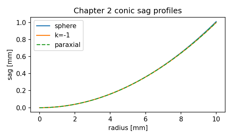
Source and validation note
The prescription vocabulary in this chapter follows standard lens-design practice: radius, thickness, material, aperture, field, wavelength, conic data, and image surface settings. The simple teaching prescription is not a manufacturing prescription. Its purpose is to make the data model inspectable before full ray tracing begins. For the full publication bibliography, see appendices/SOURCES_AND_FURTHER_READING.md.
Chapter 3: Materials, Wavelengths, and Refractive Index
A lens prescription has a small column named material.
In Chapter 2, that column looked simple. One surface said N-BK7. Another said air. We treated the material as the medium after the surface, and that was enough to prepare for ray tracing.
But the material column is not just a label.
It is a promise.
When a ray reaches a surface, the program must eventually ask:
What is the refractive index before the surface?
What is the refractive index after the surface?
At this wavelength?
The last phrase is the trap.
Not:
What is the refractive index?
but:
What is the refractive index at this wavelength?
That one condition changes everything.
A glass does not bend all colors by the same amount. Blue light and red light see slightly different refractive indices. That difference is called dispersion. Dispersion is the reason prisms spread white light into colors. It is also one of the reasons lenses have chromatic aberration. A lens that focuses green light neatly may bring blue and red light to slightly different positions.
This is not a side detail. It enters the computation early.
The full chain from Chapter 1 was:
lens prescription
→ surfaces and materials
→ real ray tracing
→ paraxial reference
→ pupil sampling
→ optical path difference
→ pupil function
→ point spread function
→ optical transfer function
→ modulation transfer function
This chapter lives in the second link:
surfaces and materials
Before we can trace a ray through glass, we need to know what the glass means numerically. Before we can compute refraction, we need n_before and n_after. Before we can compare wavelengths, we need a function that turns wavelength into refractive index.
So this chapter has one main job:
Turn the material column into a wavelength-dependent refractive index function.
We will begin with the physical idea, then write a small Python material model, then compare it with how a real optical library handles materials.
The same glass is not the same number at every wavelength
Imagine a simple singlet lens made from N-BK7.
If you ask, “What is the refractive index of N-BK7?” you may see a familiar answer:
n_d ≈ 1.5168
That number is useful, but it is incomplete.
The subscript matters. The d in n_d refers to a reference spectral line near 587.6 nm. In optical glass catalogs, refractive index is often reported at named wavelengths. The value 1.5168 does not mean “N-BK7 is always 1.5168.” It means approximately:
N-BK7 has refractive index about 1.5168 at the d-line wavelength.
At a shorter wavelength, such as blue light near 486.1 nm, the refractive index is slightly larger. At a longer wavelength, such as red light near 656.3 nm, it is slightly smaller.
That may sound like a tiny change. It is tiny numerically. But lenses are built from tiny angular changes accumulated through surfaces. A small change in refractive index can move the focus, change aberrations, and alter image quality.
The first rule of this chapter is therefore simple:
In optical computation, a material is not just a name. It is a function of wavelength.
In code, we want this shape:
n = refractive_index(material_name, wavelength_um)
or, better:
n = material.n(wavelength_um)
That is the small computational object we need.
Why wavelength units deserve respect
Before writing formulas, we need to settle units.
Optical design commonly uses:
lens distances: millimeters
wavelengths: micrometers
spatial frequency: cycles per millimeter
That mixture is normal, but it is dangerous if we forget it.
A wavelength of 587.6 nm is:
587.6 nm = 0.5876 µm = 0.0005876 mm
The same physical wavelength can be written three ways. A Python float does not know which one you meant.
For the material calculations in this book, we will use micrometers for wavelength:
wavelength_um = 0.5876
This convention is not arbitrary. Many optical glass dispersion formulas are written with wavelength in micrometers. Current Optiland material documentation also specifies wavelength inputs in microns for material refractive-index calls. (Optiland)
So when we write:
wavelength_um = 0.5876
we mean the d-line neighborhood, not half a millimeter and not 0.5876 nanometers.
This sounds fussy. It is not. Unit mistakes in optics often produce numbers that look plausible for a while. Then the result fails three chapters later, and the bug hides inside a harmless-looking 0.55.
Let us be kind to ourselves and name the unit.
Start with the wrong model on purpose
The simplest possible material model is a constant refractive index:
class ConstantMaterial:
    def __init__(self, n):
        self.n_value = float(n)

    def n(self, wavelength_um):
        return self.n_value
Use it like this:
air = ConstantMaterial(1.0)
glass = ConstantMaterial(1.5168)

for wl in [0.4861, 0.5876, 0.6563]:
    print(wl, glass.n(wl))
The output is:
0.4861 1.5168
0.5876 1.5168
0.6563 1.5168
This model is not physically correct for real glass. It says the material has the same refractive index for blue, yellow-green, and red light.
So why write it?
Because it is the correct baseline.
Many optical programs support some version of an ideal material with fixed refractive index. It is useful for testing geometry, debugging ray tracing, and building simple examples. Optiland’s material tutorial, for example, includes an IdealMaterial with fixed refractive index and extinction coefficient. (Optiland)
A constant-index material is not wrong because it is simple. It is wrong only if we forget what simplification we made.
That distinction matters.
In computation, simplifications are allowed. Silent simplifications are dangerous.
Refractive index as a curve
Now we want a material whose refractive index changes with wavelength.
For normal optical glasses in the visible region, refractive index usually decreases as wavelength increases. Blue light sees a higher index than red light. This is called normal dispersion.
A crude toy model might look like this:
class ToyDispersiveMaterial:
    def __init__(self, n_ref=1.5168, wavelength_ref_um=0.5876, slope=-0.02):
        self.n_ref = float(n_ref)
        self.wavelength_ref_um = float(wavelength_ref_um)
        self.slope = float(slope)

    def n(self, wavelength_um):
        return self.n_ref + self.slope * (wavelength_um - self.wavelength_ref_um)
Then:
toy_glass = ToyDispersiveMaterial()

for wl in [0.4861, 0.5876, 0.6563]:
    print(wl, toy_glass.n(wl))
This gives a refractive index that is higher at shorter wavelengths and lower at longer wavelengths. That is directionally useful, but not a real glass model.
We can plot it:
import numpy as np
import matplotlib.pyplot as plt

toy_glass = ToyDispersiveMaterial()
wavelengths = np.linspace(0.45, 0.70, 200)
indices = [toy_glass.n(wl) for wl in wavelengths]

plt.plot(wavelengths, indices)
plt.xlabel("wavelength [µm]")
plt.ylabel("refractive index")
plt.title("Toy dispersion model")
plt.show()
This graph is worth a pause.
The material column in the prescription is no longer a label. It has become a curve.
Later, when we trace rays, a blue ray and a red ray passing through the same lens surface will use different n_after values. That means they will refract by different amounts. That means they may focus differently.
The curve is where chromatic behavior enters the computation.
The Sellmeier equation
Real optical glass catalogs commonly use dispersion formulas. One of the most common is the Sellmeier equation.
For a three-term Sellmeier model:
n²(λ) = 1
      + B₁ λ² / (λ² - C₁)
      + B₂ λ² / (λ² - C₂)
      + B₃ λ² / (λ² - C₃)
Here:
n(λ) = refractive index at wavelength λ
λ    = wavelength, usually in micrometers for optical glass coefficients
Bᵢ   = Sellmeier B coefficients
Cᵢ   = Sellmeier C coefficients, usually in µm²
The formula looks more intimidating than the idea. It is still just a function:
wavelength → refractive index
The coefficients are fitted to measured material behavior. Different glasses have different coefficients. Once the coefficients are known, a program can compute refractive index at many wavelengths.
Let us implement it.
import math

class SellmeierMaterial:
    def __init__(self, B, C, name="unnamed"):
        self.B = tuple(float(x) for x in B)
        self.C = tuple(float(x) for x in C)
        self.name = name

    def n(self, wavelength_um):
        lam2 = wavelength_um * wavelength_um
        n2 = 1.0

        for B_i, C_i in zip(self.B, self.C):
            n2 += B_i * lam2 / (lam2 - C_i)

        return math.sqrt(n2)
For N-BK7, a commonly listed SCHOTT Sellmeier coefficient set is:
B1 = 1.039612120
B2 = 0.231792344
B3 = 1.010469450

C1 = 0.006000699
C2 = 0.0200179144
C3 = 103.56065300
SCHOTT’s N-BK7 datasheet lists these dispersion constants, with values such as n_d = 1.51680 and Abbe number ν_d = 64.17 for the glass. (Schott Media)
Now write the glass:
N_BK7 = SellmeierMaterial(
    B=(1.039612120, 0.231792344, 1.010469450),
    C=(0.006000699, 0.0200179144, 103.56065300),
    name="N-BK7",
)

for wl in [0.4861327, 0.5875618, 0.6562725]:
    print(f"{wl:.7f} µm  n = {N_BK7.n(wl):.7f}")
The exact printed values depend on rounding, but you should see the expected pattern:
blue/F-line: higher n
d-line:      middle n
red/C-line:  lower n
That pattern is dispersion.
Plotting real dispersion
Now plot the refractive index curve.
import numpy as np
import matplotlib.pyplot as plt

wavelengths = np.linspace(0.40, 0.75, 400)
indices = [N_BK7.n(wl) for wl in wavelengths]

plt.plot(wavelengths, indices)
plt.xlabel("wavelength [µm]")
plt.ylabel("refractive index")
plt.title("N-BK7 refractive index from Sellmeier equation")
plt.show()
The curve slopes downward from blue to red.
The slope is gentle, but optical systems care about gentle slopes. A lens surface does not ask whether a number looks dramatic. It uses the number in Snell’s law. A tiny index difference becomes a tiny angular difference. After propagation, that angular difference becomes a longitudinal or transverse color error. Across multiple surfaces, it becomes part of the design problem.
This is why achromatic doublets exist. A single glass has dispersion. Pairing glasses with different dispersion properties allows a designer to reduce color error. We are not designing achromats yet, but the reason they exist is already visible in this curve.
Abbe number: a compact dispersion summary
Glass catalogs need a compact way to describe dispersion. One common summary is the Abbe number.
For the d-line convention:
V_d = (n_d - 1) / (n_F - n_C)
where:
n_d = refractive index at the helium d-line, about 587.6 nm
n_F = refractive index at the hydrogen F-line, about 486.1 nm
n_C = refractive index at the hydrogen C-line, about 656.3 nm
Optiland’s material API describes the same V_d definition using the d, F, and C spectral lines. (Optiland)
Let us compute it.
F_LINE_UM = 0.4861327
D_LINE_UM = 0.5875618
C_LINE_UM = 0.6562725

def abbe_number_vd(material):
    n_F = material.n(F_LINE_UM)
    n_d = material.n(D_LINE_UM)
    n_C = material.n(C_LINE_UM)
    return (n_d - 1.0) / (n_F - n_C)

print(abbe_number_vd(N_BK7))
For N-BK7, the result should be close to 64.17, depending on coefficient precision and rounding.
What does this number mean?
A higher Abbe number means lower dispersion. A lower Abbe number means stronger dispersion.
Crown glasses often have relatively high Abbe numbers. Flint glasses often have lower Abbe numbers and higher dispersion. That distinction is central to traditional color correction.
But we should be careful.
The Abbe number is a summary, not a full refractive-index model. It uses three wavelengths to describe a curve. That is useful for classification, comparison, and approximate modeling. It is not the same as having the full dispersion curve.
This is a recurring theme in optical computation:
A compact parameter is useful only if you remember what it compresses.
An Abbe number does not replace n(λ). It gives one important clue about it.
Wavelength sets and weights
A real optical design is usually not evaluated at only one wavelength.
A simple visible-light system may use three wavelengths:
blue:  0.4861 µm
green: 0.5876 µm
red:   0.6563 µm
A more realistic imaging design may use several wavelengths with weights. The weights tell the software how much each wavelength matters in a particular analysis or optimization.
A crude example:
wavelength [µm]   weight
0.4861            0.5
0.5876            1.0
0.6563            0.5
This does not mean the green ray is “more real.” It means the design evaluation gives more importance to that wavelength.
Weights can represent a simplified spectral distribution, sensor response, photopic eye response, design priority, or just a practical engineering choice. The meaning depends on the system.
For our teaching code, we can represent wavelengths like this:
from dataclasses import dataclass

@dataclass
class Wavelength:
    value_um: float
    weight: float = 1.0
    is_primary: bool = False

wavelengths = [
    Wavelength(0.4861327, weight=0.5),
    Wavelength(0.5875618, weight=1.0, is_primary=True),
    Wavelength(0.6562725, weight=0.5),
]
Then we can evaluate material indices:
for wl in wavelengths:
    n = N_BK7.n(wl.value_um)
    marker = " primary" if wl.is_primary else ""
    print(f"{wl.value_um:.7f} µm  weight={wl.weight:.2f}  n={n:.7f}{marker}")
This is a small data structure, but it is the beginning of polychromatic optical calculation.
Later, when we compute spot diagrams, we may trace rays at multiple wavelengths and plot them in different colors. When we compute MTF, we may compute a weighted polychromatic result. When we optimize a lens, the merit function may include errors at multiple wavelengths.
Again, the later plot begins here.
Updating the lens system from Chapter 2
In Chapter 2, our LensSystem stored wavelengths as a simple list of floats:
wavelengths_um = [0.5876]
Now we can be more explicit:
from dataclasses import dataclass, field
from typing import List, Optional
import math

@dataclass
class Wavelength:
    value_um: float
    weight: float = 1.0
    is_primary: bool = False

@dataclass
class Surface:
    radius: float
    thickness: float
    material_after: str = "air"
    semi_diameter: Optional[float] = None
    conic: float = 0.0
    is_stop: bool = False
    surface_type: str = "spherical"
    comment: str = ""

    @property
    def curvature(self):
        if math.isinf(self.radius):
            return 0.0
        return 1.0 / self.radius

@dataclass
class LensSystem:
    surfaces: List[Surface] = field(default_factory=list)
    wavelengths: List[Wavelength] = field(default_factory=list)
    units: str = "mm"

    def add_surface(self, surface):
        self.surfaces.append(surface)

    def add_wavelength(self, value_um, weight=1.0, is_primary=False):
        self.wavelengths.append(Wavelength(value_um, weight, is_primary))
Now we need a material library.
class MaterialLibrary:
    def __init__(self):
        self._materials = {}

    def add(self, name, material):
        self._materials[name] = material

    def n(self, name, wavelength_um):
        if name == "air":
            return 1.0

        if name not in self._materials:
            raise ValueError(f"Unknown material: {name}")

        return self._materials[name].n(wavelength_um)
Register N-BK7:
materials = MaterialLibrary()
materials.add("N-BK7", N_BK7)
Build the singlet again:
lens = LensSystem()

lens.add_surface(Surface(
    radius=float("inf"),
    thickness=float("inf"),
    material_after="air",
    surface_type="object",
    comment="object at infinity",
))

lens.add_surface(Surface(
    radius=+50.0,
    thickness=5.0,
    material_after="N-BK7",
    semi_diameter=10.0,
    is_stop=True,
    comment="front lens surface",
))

lens.add_surface(Surface(
    radius=-50.0,
    thickness=45.0,
    material_after="air",
    semi_diameter=10.0,
    comment="back lens surface",
))

lens.add_surface(Surface(
    radius=float("inf"),
    thickness=0.0,
    material_after="air",
    surface_type="image",
    comment="image plane",
))

lens.add_wavelength(0.4861327, weight=0.5)
lens.add_wavelength(0.5875618, weight=1.0, is_primary=True)
lens.add_wavelength(0.6562725, weight=0.5)
Now ask for material transitions at each physical surface and wavelength.
def material_before_after(lens, surface_index, starting_material="air"):
    if surface_index == 0:
        before = starting_material
    else:
        before = lens.surfaces[surface_index - 1].material_after

    after = lens.surfaces[surface_index].material_after
    return before, after

for wl in lens.wavelengths:
    print(f"\nWavelength {wl.value_um:.7f} µm")
    for i, surface in enumerate(lens.surfaces):
        if surface.surface_type in ("object", "image"):
            continue

        before, after = material_before_after(lens, i)
        n_before = materials.n(before, wl.value_um)
        n_after = materials.n(after, wl.value_um)

        print(
            f"surface {i}: {before:>6} n={n_before:.7f} "
            f"→ {after:>6} n={n_after:.7f}"
        )
This is still not ray tracing, but it is now ready for ray tracing.
At each surface, for each wavelength, the program can obtain n_before and n_after.
That is exactly what the refraction algorithm will need in Chapter 6.
Snell’s law is waiting for these numbers
We are not deriving vector refraction yet. That deserves its own chapter. But we can preview why the index function matters.
Scalar Snell’s law says:
n₁ sin θ₁ = n₂ sin θ₂
where:
n₁ = refractive index before the surface
n₂ = refractive index after the surface
θ₁ = incident angle relative to the surface normal
θ₂ = refracted angle relative to the surface normal
If n₂ changes with wavelength, then θ₂ changes with wavelength.
Let us compute a tiny example. Suppose a ray in air enters N-BK7 at an incident angle of 10 degrees.
import math

def refracted_angle_deg(theta1_deg, n1, n2):
    theta1 = math.radians(theta1_deg)
    s2 = n1 * math.sin(theta1) / n2

    if abs(s2) > 1.0:
        return None  # total internal reflection

    theta2 = math.asin(s2)
    return math.degrees(theta2)

theta1_deg = 10.0

for wl in [F_LINE_UM, D_LINE_UM, C_LINE_UM]:
    n2 = N_BK7.n(wl)
    theta2 = refracted_angle_deg(theta1_deg, n1=1.0, n2=n2)
    print(f"{wl:.7f} µm  n={n2:.7f}  theta2={theta2:.6f} degrees")
The differences in refracted angle will be small. That is fine. Small differences are real.
A lens contains curved surfaces. Rays enter at different heights. The local surface normal changes. The ray propagates after refraction. A small angular difference at one surface becomes a position difference at another surface or image plane.
This is the computational birth of chromatic aberration.
It does not appear later as a mysterious defect. It begins here:
n = n(λ)
Then Snell’s law uses that n.
Longitudinal color in one thin-lens approximation
A full chromatic focus calculation requires ray tracing or paraxial system calculation. We will learn both later. But a thin-lens preview can show the direction.
For a thin lens in air, a rough lensmaker-style relationship is:
1/f ≈ (n - 1) (1/R₁ - 1/R₂)
This simplified form ignores thickness and assumes the lens is in air. It is not enough for serious design, but it is enough to see the effect of dispersion.
If n changes with wavelength, then f changes with wavelength.
Let us compute that for a symmetric biconvex lens with:
R₁ = +50 mm
R₂ = -50 mm
def thin_lens_focal_length(n, R1, R2):
    power = (n - 1.0) * (1.0 / R1 - 1.0 / R2)
    return 1.0 / power

R1 = +50.0
R2 = -50.0

for wl in [F_LINE_UM, D_LINE_UM, C_LINE_UM]:
    n = N_BK7.n(wl)
    f = thin_lens_focal_length(n, R1, R2)
    print(f"{wl:.7f} µm  n={n:.7f}  f≈{f:.3f} mm")
You should see that the focal length is not exactly the same at all three wavelengths.
This is not our final model. It is a preview of a fact the ray tracer will later show in a more direct way:
A single-element lens does not bring all wavelengths to the same focus.
Now the cause is visible: the material curve enters the refraction calculation.
A material can also absorb light
So far, we have talked only about refractive index n.
Many material databases also describe extinction coefficient k, which relates to absorption. In a complex refractive index:
N = n + i k
the real part n controls phase velocity and refraction, while k describes loss.
For the geometric ray tracing chapters that come next, we will mostly use n. But it is useful to know that a richer material model may also know about absorption. Optiland’s material classes include both refractive-index and extinction-coefficient methods, and its material tutorial demonstrates computing both n and k versus wavelength. (Optiland)
We will not build absorption into the ray tracer yet. That would distract from the main chain. But when we later discuss transmission, coatings, or non-visible materials, k becomes part of the story.
For now:
ray direction calculation → needs n(λ)
absorption/transmission calculation → may need k(λ)
One thing at a time.
Optiland material models
Our teaching code has two material types:
ConstantMaterial
SellmeierMaterial
A real library needs more.
Current Optiland material documentation describes several material types, including IdealMaterial, AbbeMaterial, AbbeMaterialE, and Material; its Material class connects to data from refractiveindex.info, while IdealMaterial provides fixed-index behavior and AbbeMaterial provides a model based on refractive index and Abbe number. (Optiland)
A minimal Optiland-style material check can look like this:
import numpy as np
import matplotlib.pyplot as plt

from optiland.materials import IdealMaterial, AbbeMaterial, Material

# Fixed-index material.
ideal = IdealMaterial(n=1.5, k=0)

# Approximate glass model from n_d and Abbe number.
abbe_glass = AbbeMaterial(n=1.5168, abbe=64.17, model="buchdahl")

# Database-backed material lookup.
# Depending on installed version and database contents,
# specifying reference or catalog can help disambiguate the material.
bk7 = Material("N-BK7", reference="Schott")

wavelengths = np.linspace(0.45, 0.70, 200)

plt.plot(wavelengths, ideal.n(wavelengths), label="Ideal n=1.5")
plt.plot(wavelengths, abbe_glass.n(wavelengths), label="Abbe model")
plt.plot(wavelengths, bk7.n(wavelengths), label="N-BK7 database")

plt.xlabel("wavelength [µm]")
plt.ylabel("refractive index")
plt.title("Different material models")
plt.legend()
plt.show()
This code is not meant to replace our Sellmeier implementation. It shows the same idea at library level.
The pattern is consistent:
material object → n(wavelength)
That is the interface we want to understand.
The real library may use databases, fitted formulas, caching, search rules, and backend arrays. Our teaching class uses three coefficients and a square root. The difference is important in engineering, but the conceptual contract is the same.
Material belongs to the surface transition
Let us return to the prescription.
In a sequential lens table, the material listed at a surface normally describes the medium after that surface.
For the singlet:
surface 1: material_after = N-BK7
surface 2: material_after = air
At surface 1:
n_before = n_air(λ)
n_after  = n_N-BK7(λ)
At surface 2:
n_before = n_N-BK7(λ)
n_after  = n_air(λ)
This is one of the simplest places to make a wrong ray tracer.
If you accidentally use the same material on both sides, the ray will not bend. If you swap before and after, the ray may bend in the wrong direction. If you use a constant glass index, the system will not show chromatic behavior. If you pass wavelength in nanometers to a function expecting micrometers, the result may be nonsense.
So before writing the refraction function, it is worth making material transitions explicit.
def index_transition(lens, materials, surface_index, wavelength_um):
    before_name, after_name = material_before_after(lens, surface_index)
    n_before = materials.n(before_name, wavelength_um)
    n_after = materials.n(after_name, wavelength_um)
    return n_before, n_after
Then:
for i, surface in enumerate(lens.surfaces):
    if surface.surface_type in ("object", "image"):
        continue

    n1, n2 = index_transition(lens, materials, i, D_LINE_UM)
    print(f"surface {i}: n1={n1:.7f}, n2={n2:.7f}")
This function is small, but it protects the logic of the next chapters.
A ray tracer should not be guessing which index to use. The prescription and material library should answer that question.
Primary wavelength is not the only wavelength
Optical design software often marks one wavelength as primary.
The primary wavelength may be used for layout, focus, paraxial reference, or default analysis. But that does not mean the other wavelengths are decorative. They may be essential for evaluating chromatic correction.
A common beginner mistake is to see a primary wavelength and forget the rest.
Better wording is:
The primary wavelength is the reference wavelength.
The wavelength set describes the spectral conditions to evaluate.
In code:
def primary_wavelength(lens):
    primary = [wl for wl in lens.wavelengths if wl.is_primary]

    if len(primary) != 1:
        raise ValueError("Lens should have exactly one primary wavelength.")

    return primary[0]

print(primary_wavelength(lens))
That function seems almost too strict, but strictness is helpful here. Ambiguous optical settings lead to ambiguous results.
When we later compute a spot diagram, we can choose:
trace only primary wavelength
trace all wavelengths
trace all wavelengths with weights
Those are different analyses. The program should know which one it is doing.
Wavelength weights are not magic
Suppose an MTF plot is labeled “polychromatic.”
That sounds impressive, but it still has to mean something concrete.
At some point, the program has to combine information from multiple wavelengths. It may use weights. It may use a spectral distribution. It may use sensor response. It may use a simplified user-defined set.
A simple weighted average looks like this:
def weighted_average(values, weights):
    values = np.asarray(values, dtype=float)
    weights = np.asarray(weights, dtype=float)
    return np.sum(values * weights) / np.sum(weights)
For refractive index itself, averaging is not usually the right physical operation for a lens calculation, because rays at each wavelength should be traced with their own index. But the function shows the general idea of weighted combination.
A better mental model is:
for each wavelength:
    compute the optical result using n(λ)

then:
    combine wavelength-specific results according to the analysis method
That matters for later.
A polychromatic spot diagram is not created by tracing one average wavelength. It is created by tracing multiple wavelengths and displaying or combining their ray intersections. A polychromatic MTF is not made by pretending the glass has one average index. It requires wavelength-aware computation before the final combination.
This is a place where software commands can hide a lot.
The button may say:
Polychromatic MTF
The computation says:
wavelength set
→ material indices at each wavelength
→ ray or wavefront calculation at each wavelength
→ wavelength-specific image-quality result
→ weighted combination
We are not ready to compute that full chain yet. But now we know where it begins.
Common mistakes with materials and wavelengths
Let us collect the mistakes now, while they are still easy to see.
Mistake 1: Treating refractive index as a universal constant
N-BK7 ≈ 1.5168 is not a complete material model. It is a reference value near the d-line.
Use constant index when you intentionally want a simplified model. Do not use it accidentally.
Mistake 2: Passing wavelength in the wrong unit
A function expecting micrometers should receive:
0.5876
not:
587.6
unless the function explicitly expects nanometers.
This is one of the easiest ways to ruin a calculation quietly.
Mistake 3: Confusing Abbe number with full dispersion
The Abbe number summarizes dispersion using selected wavelengths. It is useful, but it is not the whole refractive-index curve.
Mistake 4: Forgetting that material is “after surface”
In a sequential prescription, the material listed at surface i usually describes the medium after surface i.
The refraction at a surface needs both sides:
previous material → current material_after
Mistake 5: Averaging refractive indices too early
For multi-wavelength analysis, do not replace all wavelengths with one average refractive index unless that is a deliberate approximation. Trace or compute each wavelength according to the analysis being performed.
Mistake 6: Ignoring valid wavelength range
Dispersion formulas are valid over specified wavelength ranges. Extrapolating outside that range can produce wrong results. Real material databases usually carry range information for a reason.
Mistake 7: Forgetting air is also a material
For many visible-light teaching examples, we treat air as n = 1.0. In high-precision work, air itself has wavelength-, temperature-, pressure-, and humidity-dependent refractive index. We will use 1.0 for now because it keeps the early ray tracer focused. But it is still a model choice.
What this chapter adds to the computation chain
In Chapter 2, we could say:
surface 1 has material N-BK7
Now we can say:
surface 1 changes the medium from air to N-BK7

at λ = 0.4861 µm:
    n_before = 1.0
    n_after  = n_N-BK7(0.4861)

at λ = 0.5876 µm:
    n_before = 1.0
    n_after  = n_N-BK7(0.5876)

at λ = 0.6563 µm:
    n_before = 1.0
    n_after  = n_N-BK7(0.6563)
That is a real improvement.
The prescription is no longer only geometry. It now contains wavelength-dependent optical behavior.
Our computational chain has become:
surface table
→ material names
→ material models
→ refractive index n(λ)
→ index transition at each surface
→ ready for Snell refraction
This is exactly the missing piece before we define rays.
A small final test
Let us write one compact test that confirms the chapter’s work.
def print_surface_indices(lens, materials):
    for wl in lens.wavelengths:
        print(f"\nλ = {wl.value_um:.7f} µm, weight = {wl.weight}")
        for i, s in enumerate(lens.surfaces):
            if s.surface_type in ("object", "image"):
                continue

            before, after = material_before_after(lens, i)
            n1 = materials.n(before, wl.value_um)
            n2 = materials.n(after, wl.value_um)

            print(
                f"surface {i}: {before} → {after}, "
                f"n1={n1:.7f}, n2={n2:.7f}"
            )

print_surface_indices(lens, materials)
If this prints different N-BK7 indices for different wavelengths, the material system is doing its job.
It is not tracing rays yet. It is preparing the numbers that ray tracing needs.
That is enough.
The road ahead
We now have:
a lens prescription as data
surface geometry
material names
wavelength settings
a refractive-index function n(λ)
index transitions at each surface
The next object is the ray itself.
A ray is not a vague line in a drawing. In code, it must have a position, a direction, a wavelength, perhaps intensity, perhaps status flags, and eventually optical path length. It must be able to propagate. It must be able to meet surfaces. It must carry the wavelength that tells the material library which refractive index to use.
So Chapter 4 will ask a plain question:
What is a ray in code?
Once we answer that, the pieces will begin to move.
The lens prescription gives the world.
The material model gives each medium its wavelength-dependent behavior.
The ray will be the traveler.
Generated validation figure
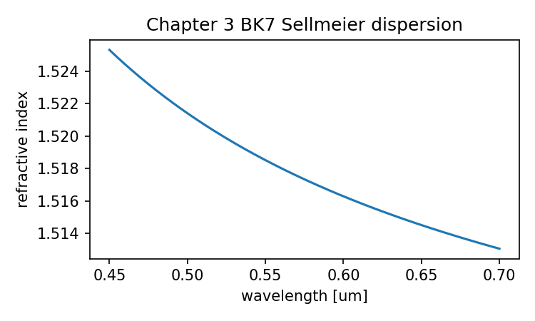
Source and validation note
The wavelength-dependent material discussion should be read against glass-catalog and optical-constants sources, not only against the simplified teaching code. In the companion validation, BK7 dispersion is generated for teaching purposes; production work should use a catalog source and record the exact glass vendor, reference data, wavelength unit, and temperature assumptions.
Chapter 4: How to Represent a Ray
A ray in an optical drawing looks effortless.
It is just a line.
It leaves the object, passes through the lens, bends at the surfaces, and lands near the image plane. If several rays are drawn together, they form a neat fan. If they are traced through a good lens, they gather. If the lens is poor, they spread. The picture is intuitive enough that we may forget a simple fact:
A drawn ray is not yet a computational ray.
A program cannot trace a sketch. It needs numbers.
It needs to know where the ray starts, which direction it travels, what wavelength it carries, whether it is still valid, and eventually how much optical path length it has accumulated. If we want to build spot diagrams, wavefront maps, PSF, and MTF from first principles, we must first make this object explicit.
This chapter is about that object.
Not the surface yet. Not refraction yet. Not the image quality yet.
Just the ray.
That may feel like a small topic, but it is the root of everything that follows. A ray tracer is not a magic optical engine. It is a loop that repeatedly performs a few operations on a ray:
start with a ray
→ find where it hits the next surface
→ compute the surface normal
→ refract or reflect the ray
→ propagate to the next surface
→ repeat
If the ray itself is vague, the loop becomes vague.
So let us make the ray concrete.
A ray is a parametric line with optical baggage
The basic geometric form of a ray is:
r(t) = r0 + t d
Here:
r0 = starting point of the ray
d  = direction vector
t  = distance-like parameter along the ray
If d is normalized so that its length is 1, then t has the same length unit as the coordinates. If positions are in millimeters, then t is in millimeters.
This is a very useful convention.
For example, if:
r0 = [0, 0, 0]
d  = [0, 0, 1]
then:
r(10) = [0, 0, 10]
The ray has moved 10 mm in the positive z direction.
If the ray is tilted:
d = [0.1, 0, 0.995]
then moving forward changes both x and z.
This is the geometry. But an optical ray needs more than geometry. It should also carry at least:
wavelength
intensity
optical path length
valid / invalid status
Later, a more advanced ray may also carry polarization state, phase, surface history, or differential information for optimization. We do not need all of that yet.
For now, our ray will know five things:
position
direction
wavelength
intensity
optical path length
and one status flag:
alive or stopped
That is enough to begin.
Normalize the direction, always
The direction vector should be normalized.
That means:
||d|| = 1
or:
sqrt(dx² + dy² + dz²) = 1
Why insist on this?
Because it makes propagation clean. If d has unit length, then t is physical distance. Moving the ray by t = 5.0 means moving it 5.0 mm through space.
If d is not normalized, then t becomes harder to interpret. A ray with direction [0, 0, 10] and a ray with direction [0, 0, 1] point the same way, but r0 + t d moves them by very different amounts for the same t.
That is not what we want.
So the ray constructor should normalize the direction immediately.
import numpy as np

def normalize(v):
    """Return a unit-length copy of vector v."""
    v = np.asarray(v, dtype=float)
    norm = np.linalg.norm(v)

    if norm == 0:
        raise ValueError("Cannot normalize a zero vector.")

    return v / norm
Test it:
d = normalize([0, 0, 10])
print(d)
print(np.linalg.norm(d))
The result is:
[0. 0. 1.]
1.0
This tiny helper function will appear everywhere. It is one of the quiet tools that keeps ray tracing stable.
A first Ray class
Let us write a minimal Ray class.
from dataclasses import dataclass, field
import numpy as np

@dataclass
class Ray:
    position: np.ndarray
    direction: np.ndarray
    wavelength_um: float = 0.5876
    intensity: float = 1.0
    opl: float = 0.0
    alive: bool = True
    stop_reason: str = ""
    history: list = field(default_factory=list)

    def __post_init__(self):
        self.position = np.asarray(self.position, dtype=float)
        self.direction = normalize(self.direction)

        if self.position.shape != (3,):
            raise ValueError("Ray position must be a 3D vector.")

        if self.direction.shape != (3,):
            raise ValueError("Ray direction must be a 3D vector.")

        if self.wavelength_um <= 0:
            raise ValueError("Wavelength must be positive.")

        if self.intensity < 0:
            raise ValueError("Intensity cannot be negative.")

    def point_at(self, t):
        """Return the point r(t) = r0 + t d."""
        return self.position + t * self.direction

    def copy(self):
        """Return a copy of the ray."""
        return Ray(
            position=self.position.copy(),
            direction=self.direction.copy(),
            wavelength_um=self.wavelength_um,
            intensity=self.intensity,
            opl=self.opl,
            alive=self.alive,
            stop_reason=self.stop_reason,
            history=list(self.history),
        )
This is not yet a ray tracer. It is a well-defined object that a ray tracer can use.
A ray has a position and a direction. It knows its wavelength. It has an intensity. It has an accumulated optical path length, opl. It can be alive or stopped. It can store history if we want to inspect where it has been.
Now create a ray:
ray = Ray(
    position=[0.0, 0.0, 0.0],
    direction=[0.1, 0.0, 1.0],
    wavelength_um=0.5876,
)

print("position:", ray.position)
print("direction:", ray.direction)
print("direction length:", np.linalg.norm(ray.direction))
print("point at t=10:", ray.point_at(10.0))
The direction is automatically normalized. The point at t = 10 lies 10 mm along that normalized direction.
This is the first real computational ray.
The direction vector is not the same as an angle
In simple two-dimensional drawings, we often describe rays by an angle.
For example:
a ray tilted by 5 degrees from the optical axis
That is fine for human discussion. But in three-dimensional computation, a direction vector is often more convenient.
A direction vector can represent tilt in both x and y. It also works naturally with dot products, surface normals, vector refraction, and intersections.
Still, it is useful to create a direction from angles.
Let the optical axis be the positive z axis. A ray tilted in the x-z plane by angle θx has direction:
d = [sin θx, 0, cos θx]
For small field angles, this is enough.
import math

def direction_from_x_angle(theta_x_deg):
    """Create a unit direction vector tilted in the x-z plane."""
    theta = math.radians(theta_x_deg)
    return np.array([math.sin(theta), 0.0, math.cos(theta)])

for angle in [0.0, 5.0, 10.0]:
    print(angle, direction_from_x_angle(angle))
For tilts in both x and y, we can write a simple helper. One clean construction is to point the ray toward a plane at z = 1:
def direction_from_field_angles(theta_x_deg=0.0, theta_y_deg=0.0):
    """Create a direction vector from approximate field angles.

    The ray points toward (tan θx, tan θy, 1).
    This is convenient for field-angle based examples.
    """
    tx = math.tan(math.radians(theta_x_deg))
    ty = math.tan(math.radians(theta_y_deg))
    return normalize([tx, ty, 1.0])
Test it:
print(direction_from_field_angles(0.0, 0.0))
print(direction_from_field_angles(5.0, 0.0))
print(direction_from_field_angles(0.0, 5.0))
print(direction_from_field_angles(5.0, 5.0))
This helper is not a full field model. It is just a practical way to generate rays that travel roughly along the optical axis with a specified angular tilt.
Later, when we generate bundles of rays from field points and pupil coordinates, this kind of function will become part of a larger sampling routine.
Propagating a ray by distance
The simplest operation on a ray is propagation through a uniform medium.
If the ray moves a physical distance s, its new position is:
r_new = r_old + s d
If the medium has refractive index n, the optical path length increases by:
ΔOPL = n s
This deserves attention.
Geometric distance and optical path length are not the same thing. A ray traveling 10 mm through air has optical path length about 10 mm if n ≈ 1. The same geometric distance through glass with n = 1.5 has optical path length about 15 mm.
This will matter later when we compute OPD. Wavefront error is not built from plain geometric distance alone. It depends on optical path.
Let us implement propagation.
@dataclass
class Ray:
    position: np.ndarray
    direction: np.ndarray
    wavelength_um: float = 0.5876
    intensity: float = 1.0
    opl: float = 0.0
    alive: bool = True
    stop_reason: str = ""
    history: list = field(default_factory=list)

    def __post_init__(self):
        self.position = np.asarray(self.position, dtype=float)
        self.direction = normalize(self.direction)

        if self.position.shape != (3,):
            raise ValueError("Ray position must be a 3D vector.")
        if self.direction.shape != (3,):
            raise ValueError("Ray direction must be a 3D vector.")
        if self.wavelength_um <= 0:
            raise ValueError("Wavelength must be positive.")
        if self.intensity < 0:
            raise ValueError("Intensity cannot be negative.")

    def point_at(self, t):
        return self.position + t * self.direction

    def propagate(self, distance, refractive_index=1.0):
        """Move the ray forward by geometric distance.

        distance is in the same length unit as position, usually mm.
        refractive_index is dimensionless.
        """
        if not self.alive:
            return self

        if distance < 0:
            raise ValueError("Propagation distance should be non-negative.")

        old_position = self.position.copy()
        self.position = self.point_at(distance)
        self.opl += refractive_index * distance

        self.history.append({
            "event": "propagate",
            "from": old_position,
            "to": self.position.copy(),
            "distance": distance,
            "n": refractive_index,
            "opl": self.opl,
        })

        return self

    def stop(self, reason):
        self.alive = False
        self.stop_reason = reason
        self.history.append({
            "event": "stop",
            "reason": reason,
            "position": self.position.copy(),
        })
        return self

    def copy(self):
        return Ray(
            position=self.position.copy(),
            direction=self.direction.copy(),
            wavelength_um=self.wavelength_um,
            intensity=self.intensity,
            opl=self.opl,
            alive=self.alive,
            stop_reason=self.stop_reason,
            history=list(self.history),
        )
Now try it:
ray = Ray([0, 0, 0], [0, 0, 1], wavelength_um=0.5876)
ray.propagate(10.0, refractive_index=1.0)

print(ray.position)
print(ray.opl)
The output is:
[ 0.  0. 10.]
10.0
Through glass:
ray = Ray([0, 0, 0], [0, 0, 1], wavelength_um=0.5876)
ray.propagate(10.0, refractive_index=1.5)

print(ray.position)
print(ray.opl)
The position is still [0, 0, 10], but the optical path length is 15.0.
That small distinction is one of the bridges from geometric ray tracing to wavefront computation.
Propagating to a z plane
In sequential optical systems, many useful surfaces are arranged along the z axis. Even before we handle curved surfaces, it is useful to ask:
Where does this ray meet the plane z = z_target?
For a ray:
r(t) = r0 + t d
the z coordinate is:
z(t) = z0 + t dz
Set this equal to z_target:
z_target = z0 + t dz
Solve for t:
t = (z_target - z0) / dz
This formula is simple, but it already teaches an important habit: intersection is usually parameter solving. We find the parameter t that places the ray on the target surface.
Here is the code:
def distance_to_z_plane(ray, z_target, eps=1e-12):
    """Return distance parameter t where ray reaches z = z_target."""
    dz = ray.direction[2]

    if abs(dz) < eps:
        return None

    t = (z_target - ray.position[2]) / dz

    if t < 0:
        return None

    return t
Now use it:
ray = Ray([0, 0, 0], [0.1, 0.0, 1.0])
t = distance_to_z_plane(ray, 50.0)

print("distance to z=50:", t)
print("point:", ray.point_at(t))
The ray reaches the z plane at a point with nonzero x coordinate. That x coordinate is the transverse displacement caused by the ray’s tilt.
We can add a method:
def propagate_to_z(ray, z_target, refractive_index=1.0):
    t = distance_to_z_plane(ray, z_target)

    if t is None:
        ray.stop(f"Cannot reach z plane {z_target}")
        return ray

    return ray.propagate(t, refractive_index=refractive_index)
Test:
ray = Ray([0, 0, 0], direction_from_field_angles(theta_x_deg=5.0))
propagate_to_z(ray, 100.0, refractive_index=1.0)

print(ray.position)
print(ray.opl)
This is the first usable intersection-like operation in the book. It is only a plane perpendicular to the optical axis, but it introduces the core pattern:
solve for t
evaluate r(t)
update the ray
In Chapter 5, we will use the same pattern for real surfaces.
A ray can miss, go backward, or become invalid
The formula for t is not enough by itself. A ray can fail to reach a plane in the forward direction.
If dz = 0, the ray is parallel to the z plane. It never reaches a different z value.
If t < 0, the plane lies behind the ray, not in front of it.
That is why distance_to_z_plane returns None in those cases.
This is not just defensive programming. Ray tracing is full of validity checks.
A ray may be invalid because:
it misses a surface
it hits outside the clear aperture
it undergoes total internal reflection when refraction was expected
it travels backward
it encounters an unsupported surface
it loses too much intensity
Rather than pretending every ray always survives, we should make validity part of the ray object.
That is why our Ray class has:
alive
stop_reason
This will become useful when we trace a bundle of rays. Some rays will pass through the whole system. Some may be clipped. A spot diagram should normally include only rays that reach the image plane.
A ray tracer that never stops rays is not being optimistic. It is being careless.
Wavelength belongs to the ray
In Chapter 3, we built material models where refractive index depends on wavelength:
n = n(λ)
Where should λ live during ray tracing?
It should live on the ray.
A blue ray and a red ray may start from the same point and travel in the same initial direction. But when they hit glass, the material library will give them different refractive indices. That means refraction may send them in slightly different directions.
So the ray must carry its wavelength:
blue_ray = Ray([0, 0, 0], [0, 0, 1], wavelength_um=0.4861327)
green_ray = Ray([0, 0, 0], [0, 0, 1], wavelength_um=0.5875618)
red_ray = Ray([0, 0, 0], [0, 0, 1], wavelength_um=0.6562725)
Later, at a surface, the tracing code can ask:
n_before = materials.n(before_material, ray.wavelength_um)
n_after = materials.n(after_material, ray.wavelength_um)
That is how the material chapter connects to the ray chapter.
The lens prescription says which materials appear after which surfaces. The material library says how each material behaves at each wavelength. The ray carries the wavelength that selects the correct refractive index.
The pieces are beginning to fit.
Intensity belongs to the ray too
For early geometric ray tracing, intensity may seem unnecessary. Many simple ray traces only care where rays go.
But intensity is useful to include from the beginning because real optical calculations often need to know whether rays are weighted equally.
A ray may carry lower intensity because:
it belongs to a weighted wavelength
it comes from a weighted pupil sample
it passes through a partially transmitting element
it reflects or absorbs at a surface
We will not model coatings or absorption yet. But an intensity field costs almost nothing and makes the ray object more honest.
A simple rule for now:
intensity = 1.0 means full weight
intensity = 0.0 means no contribution
When we generate a ray bundle later, we may assign weights to rays according to pupil sampling or wavelength weights. That will matter when summing results.
Again, not all fields are used immediately. A good data structure prepares for the next steps without becoming bloated.
Optical path length is not optional forever
A beginner ray tracer can ignore optical path length if it only wants spot diagrams.
But this book does not stop at spot diagrams. We are heading toward OPD, wavefront, PSF, and MTF. For that path, optical path length matters.
When a ray travels a distance s through refractive index n, it accumulates:
OPL += n s
For a sequence of media:
OPL = n1 s1 + n2 s2 + n3 s3 + ...
This looks harmless. But later, OPD will compare optical path lengths across rays. That comparison is one of the main bridges from ray tracing to wave optics.
So our ray stores opl from the start.
Even if we do not fully use it until Chapter 10, the habit is important:
A ray is not only a line. It is also a path through optical media.
The geometry tells us where it goes.
The OPL tells us how much optical distance it has traveled.
Ray history is for learning, not always for production
Our Ray class stores a history list. Every propagation event can append a small record.
This is helpful for learning and debugging:
ray = Ray([0, 0, 0], [0.05, 0, 1])
ray.propagate(10.0, refractive_index=1.0)
ray.propagate(5.0, refractive_index=1.5)

for event in ray.history:
    print(event)
A production ray tracer may avoid storing full history for every ray because it can be expensive. If you trace millions of rays, memory matters.
But for a teaching implementation, history is lovely. It lets us inspect the path instead of trusting the final answer. This matches the spirit of the book: we are not trying to hide the computation. We are trying to see it.
Later, if performance becomes important, we can turn history off.
For now, clarity wins.
A small ray table
Let us generate a few rays and propagate them to the same z plane.
rays = [
    Ray([0, 0, 0], direction_from_field_angles(theta_x_deg=0.0)),
    Ray([0, 0, 0], direction_from_field_angles(theta_x_deg=2.0)),
    Ray([0, 0, 0], direction_from_field_angles(theta_x_deg=-2.0)),
]

z_image = 100.0

for ray in rays:
    propagate_to_z(ray, z_image)
    print(
        f"angle-like direction={ray.direction}, "
        f"hit position={ray.position}, "
        f"OPL={ray.opl:.3f}"
    )
The on-axis ray lands at x = 0. The tilted rays land on opposite sides.
This is not a lens yet. It is free-space propagation. But even here we can see the beginning of a spot diagram: a collection of ray landing points.
Let us plot them.
import matplotlib.pyplot as plt

xs = [ray.position[0] for ray in rays]
ys = [ray.position[1] for ray in rays]

plt.scatter(xs, ys)
plt.axhline(0, linewidth=0.5)
plt.axvline(0, linewidth=0.5)
plt.xlabel("x at z plane [mm]")
plt.ylabel("y at z plane [mm]")
plt.title("Ray landing points on a z plane")
plt.gca().set_aspect("equal", adjustable="box")
plt.show()
This is a very boring spot diagram. Good. Boring diagrams are sometimes the best starting point.
Nothing has refracted yet. No surface has been hit. No aberration exists. We are only confirming that rays can move, carry their properties, and land somewhere measurable.
From one ray to many rays
Most optical analysis does not trace only one ray.
It traces bundles.
A bundle may represent:
different heights in the pupil
different field points
different wavelengths
different object points
different sampling weights
For now, let us create a simple fan of rays in the x-z plane, all starting at the origin but with different angles.
def make_angle_fan(theta_min_deg, theta_max_deg, count, wavelength_um=0.5876):
    angles = np.linspace(theta_min_deg, theta_max_deg, count)
    return [
        Ray(
            position=[0.0, 0.0, 0.0],
            direction=direction_from_field_angles(theta_x_deg=a),
            wavelength_um=wavelength_um,
        )
        for a in angles
    ]

fan = make_angle_fan(-5.0, 5.0, 11)

for ray in fan:
    propagate_to_z(ray, 100.0)

xs = [ray.position[0] for ray in fan]
ys = [ray.position[1] for ray in fan]

plt.scatter(xs, ys)
plt.xlabel("x at z = 100 mm")
plt.ylabel("y at z = 100 mm")
plt.title("Free-space fan landing points")
plt.gca().set_aspect("equal", adjustable="box")
plt.show()
The rays spread linearly because there is no lens.
Later, when we add surfaces and refraction, the same bundle will bend. After tracing through a lens, the landing points at the image plane will become a real spot diagram.
The spot diagram will not be “drawn.” It will be the result of ray objects being propagated through a system.
That is the exact mental shift we want.
Real ray and paraxial ray
Now we need to make an important distinction.
A real ray is what we have been building: a geometric ray with a full position vector and direction vector. It can hit exact surfaces. It can refract using exact normals. It does not assume small angles unless we choose to create small-angle rays.
A paraxial ray is different. It lives inside a small-angle approximation near the optical axis. Instead of full 3D geometry, paraxial optics often tracks quantities like ray height and slope:
y = ray height
u = ray angle or slope
A paraxial ray is not “fake” in the useless sense. It is a simplified model that captures the first-order skeleton of the optical system.
Real ray tracing asks:
Where does the actual ray go through the actual surface geometry?
Paraxial tracing asks:
How does a near-axis, small-angle ray behave under first-order approximations?
Both matter.
Paraxial rays help compute:
effective focal length
back focal length
principal planes
F-number
magnification
first-order layout
Real rays help compute:
aberrations
spot diagrams
ray fans
real focus behavior
field-dependent errors
In this book, we will use both. But we must not confuse them.
A tiny paraxial ray class might look like this:
@dataclass
class ParaxialRay:
    y: float      # ray height
    u: float      # small angle or slope
    wavelength_um: float = 0.5876

    def propagate(self, distance):
        """Small-angle propagation: y_new = y + distance * u."""
        self.y = self.y + distance * self.u
        return self
This is much simpler than the real Ray class. It has no 3D position, no exact direction vector, no surface intersection logic. That simplicity is useful when we study first-order optics in Chapter 8.
But the ray tracer in Chapters 5–7 will use real rays.
Here is the clean boundary:
Chapters 4–7: real ray representation and tracing
Chapter 8: paraxial ray transfer and first-order optics
Chapter 9 onward: compare real rays against paraxial reference
If you keep that boundary clear, many later topics become easier.
A ray is not a beam
Another useful distinction:
A ray is not a beam.
A ray is a geometric sample. A beam is a physical distribution of light.
When we trace many rays through a pupil, we are not claiming that each ray is a tiny physical thread of light. We are sampling the behavior of an optical system. A ray bundle is a computational representation.
This matters because different analyses use different sampling ideas.
For a spot diagram, we may trace a finite set of rays and plot their intersections.
For wavefront analysis, we may trace rays associated with pupil coordinates and compute optical path differences.
For diffraction PSF, we eventually need a pupil function, not just a list of ray landing points.
The ray is a tool. It is powerful, but it is not the whole physics of light.
That is why this book will not stop at geometric ray tracing. It will use rays to build the bridge toward wavefront and diffraction calculations.
But first, the rays must be correct.
Coordinate conventions
Let us state the coordinate convention we will use in the teaching code.
z axis: nominal optical axis
x, y: transverse coordinates
light travels generally in +z direction
positions are in millimeters
wavelengths are in micrometers
direction vectors are unitless and normalized
This is a convention, not a law of nature. Other software may use different coordinate choices or sign conventions. Professional optical design programs are very careful about these definitions.
For our purposes, this convention keeps early examples readable.
A ray starting at the origin and traveling along the optical axis is:
Ray(position=[0, 0, 0], direction=[0, 0, 1])
A ray starting 5 mm above the axis and traveling forward is:
Ray(position=[0, 5, 0], direction=[0, 0, 1])
A ray tilted in x is:
Ray(position=[0, 0, 0], direction=direction_from_field_angles(theta_x_deg=3.0))
These choices are simple enough to inspect by hand.
That is exactly what we want before adding curved surfaces.
Keeping units straight
The ray object carries both position and wavelength, but they use different units:
position: mm
wavelength: µm
This may look odd, but it follows common optical design practice.
Why not store everything in millimeters?
We could. But material dispersion formulas and glass catalogs often use wavelength in micrometers. If we keep wavelength in micrometers, our material code from Chapter 3 remains natural.
The danger is mixing them.
When computing ray propagation and surface intersection, use millimeters.
When asking a material for refractive index, pass micrometers.
When converting OPD to phase later, be careful: OPD may be in millimeters while wavelength may be in micrometers. That conversion will matter. We will handle it explicitly when we reach wavefront phase.
For now, just keep the labels clear.
A good ray object does not solve every unit problem, but it can make the unit assumptions visible.
A more careful propagation example
Let us combine wavelength, material index, and OPL.
Suppose a green ray travels:
20 mm in air
5 mm in N-BK7
20 mm in air
At the d-line, N-BK7 has index about 1.5168. The geometric distance is:
20 + 5 + 20 = 45 mm
The optical path length is about:
1.0 × 20 + 1.5168 × 5 + 1.0 × 20 = 47.584 mm
Let us compute it:
ray = Ray([0, 0, 0], [0, 0, 1], wavelength_um=0.5876)

ray.propagate(20.0, refractive_index=1.0)
ray.propagate(5.0, refractive_index=1.5168)
ray.propagate(20.0, refractive_index=1.0)

print("position:", ray.position)
print("OPL:", ray.opl)
This example is deliberately one-dimensional. It ignores refraction and assumes the ray simply travels through segments. Still, it teaches the bookkeeping.
Later, when the ray bends at surfaces, the geometric segment lengths will come from intersection calculations. The refractive index will come from the material model. The OPL will accumulate segment by segment.
The final OPD calculation will compare these accumulated paths.
So even now, the ray object is carrying future wavefront information.
Plotting a ray path
A ray history lets us draw a simple path.
def extract_path_from_history(ray):
    points = []

    for event in ray.history:
        if event["event"] == "propagate":
            if not points:
                points.append(event["from"])
            points.append(event["to"])

    return np.array(points)

ray = Ray([0, 0, 0], direction_from_field_angles(theta_x_deg=5.0))
ray.propagate(20.0)
ray.propagate(30.0)

path = extract_path_from_history(ray)

plt.plot(path[:, 2], path[:, 0], marker="o")
plt.xlabel("z [mm]")
plt.ylabel("x [mm]")
plt.title("Ray path in the x-z plane")
plt.gca().set_aspect("equal", adjustable="box")
plt.show()
We plot z horizontally and x vertically because that resembles the usual optical layout view.
This is still a straight line. That is good. Before a ray can bend correctly, it should travel straight correctly.
A surprising number of bugs in ray tracing are easier to catch if you first test boring straight-line behavior.
What a real optical library adds
Our Ray class is for learning. A real optical library must handle much more.
For example, a practical ray-tracing system may need:
arrays of many rays
multiple fields
multiple wavelengths
surface-by-surface data
aperture clipping
ray aiming
chief and marginal ray search
polarization state
vignetting factors
coordinate breaks
surface local coordinates
backend support for NumPy, PyTorch, or JAX
Optiland, as the reference library for this book, provides higher-level ray-tracing workflows inside a full optical system model. We will not try to mirror its internal ray objects line by line. That would turn this book into an API commentary, which is not the goal.
Instead, we use a two-level reading.
At the teaching-code level, a ray is transparent:
ray = Ray(position=[0, 0, 0], direction=[0, 0, 1], wavelength_um=0.5876)
At the library level, rays are usually generated and traced through an optical system:
# Schematic Optiland-style workflow.
# Exact method names may vary by version.

from optiland.samples.objectives import CookeTriplet

lens = CookeTriplet()

# The library can draw the system and trace rays for visualization.
lens.draw(num_rays=5)
This kind of call hides many details intentionally. It chooses ray samples, traces them through the surfaces, and plots the result. That is useful.
But now we know what must exist underneath:
ray position
ray direction
ray wavelength
surface intersections
material indices
refraction updates
validity checks
The exact internal organization may differ from our teaching class. The computational obligations do not disappear.
A library can make ray tracing convenient. It cannot make rays unnecessary.
A minimal ray-tracing skeleton
We can now write the skeleton of a ray tracer, even though we have not implemented surfaces yet.
def trace_ray_through_system(ray, surfaces, materials):
    """A skeleton only.

    Chapter 5 will fill in ray-surface intersection.
    Chapter 6 will fill in refraction.
    """
    for surface in surfaces:
        if not ray.alive:
            break

        # 1. Find where the ray intersects this surface.
        # intersection = intersect(ray, surface)

        # 2. If it misses, stop the ray.
        # if intersection is None:
        #     ray.stop("missed surface")
        #     break

        # 3. Propagate ray to the intersection point.
        # distance = intersection.distance
        # ray.propagate(distance, refractive_index=current_n)

        # 4. Check clear aperture.
        # if outside aperture:
        #     ray.stop("blocked by aperture")
        #     break

        # 5. Compute normal.
        # normal = surface_normal(surface, ray.position)

        # 6. Compute n_before and n_after using ray.wavelength_um.
        # n1, n2 = index_transition(...)

        # 7. Refract ray direction.
        # ray.direction = refract(ray.direction, normal, n1, n2)

        pass

    return ray
This function does not run yet. It is a map.
The important point is that the ray object already contains the information the future functions need.
intersect will use the ray’s position and direction.
index_transition will use the ray’s wavelength.
propagate will update the ray’s position and optical path length.
refract will update the ray’s direction.
A ray tracer is not one giant spell. It is a sequence of small operations with clear inputs and outputs.
Testing the Ray class
Before building more machinery on top of the ray, let us write a few small tests.
def test_direction_is_normalized():
    ray = Ray([0, 0, 0], [0, 0, 10])
    assert np.isclose(np.linalg.norm(ray.direction), 1.0)

def test_point_at():
    ray = Ray([1, 2, 3], [0, 0, 1])
    p = ray.point_at(5)
    assert np.allclose(p, [1, 2, 8])

def test_propagate_updates_position_and_opl():
    ray = Ray([0, 0, 0], [0, 0, 1])
    ray.propagate(10, refractive_index=1.5)
    assert np.allclose(ray.position, [0, 0, 10])
    assert np.isclose(ray.opl, 15.0)

def test_propagate_to_z():
    ray = Ray([0, 0, 0], [0, 0, 1])
    propagate_to_z(ray, 25.0)
    assert np.allclose(ray.position, [0, 0, 25.0])

test_direction_is_normalized()
test_point_at()
test_propagate_updates_position_and_opl()
test_propagate_to_z()

print("All ray tests passed.")
This may feel a little too software-engineering-like for an optics book. It is not.
Optical computation is software. If the basic ray object is wrong, the later optical plots may still look beautiful, but they will be wrong.
Small tests are not decoration. They are how we keep trust in the calculation.
Common mistakes when representing rays
Let us collect the traps now.
Mistake 1: Not normalizing direction
If the direction vector is not unit length, propagation distance becomes ambiguous. Normalize it at construction time.
Mistake 2: Confusing direction with endpoint
A direction vector is not a point the ray is trying to reach. It is an orientation. If you want to define a ray from point A toward point B, compute:
d = normalize(B - A)
not just d = B.
Mistake 3: Forgetting wavelength
A ray without wavelength cannot select the correct refractive index in a dispersive material.
You can use a default wavelength, but it should be explicit.
Mistake 4: Ignoring invalid rays
Some rays should stop. If you keep tracing blocked or missed rays, your later diagrams may include nonsense.
Mistake 5: Treating OPL as geometric distance
Geometric distance is s. Optical path length is n s. They are equal only when n = 1.
Mistake 6: Mixing units silently
Positions may be in millimeters while wavelengths are in micrometers. That is acceptable only if the code says so clearly.
Mistake 7: Confusing real and paraxial rays
A paraxial ray is a first-order approximation. A real ray is a geometric object traced through actual surfaces. Both are useful. They are not interchangeable.
What this chapter gives us
We now have a computational ray.
It can:
store position and direction
normalize its direction
carry wavelength and intensity
accumulate optical path length
move forward by distance
move to a z plane
stop when invalid
record history for inspection
This may not look dramatic yet. No lens has focused anything. No ray has bent. No spot diagram has appeared.
But the foundation is now solid.
The prescription from Chapter 2 gives us the optical system as data.
The material model from Chapter 3 gives us refractive index as a function of wavelength.
The ray object from this chapter gives us something that can travel through that system.
The next missing piece is the surface encounter.
A ray can move in a straight line. A lens surface sits somewhere in space. The ray tracer must answer:
At what point does this ray hit that surface?
For a plane, this is easy.
For a sphere, it becomes a quadratic equation.
For aspheres and more complex surfaces, it may require numerical methods.
That is where the real work begins.
Chapter 5 will take the ray we have built here and make it collide with geometry. We will compute ray-plane and ray-sphere intersections by hand. It is one of the most important chapters in the book, because it shows the part many explanations skip.
A ray drawing shows a line touching glass.
A ray tracer has to calculate the touch.
Generated validation figure
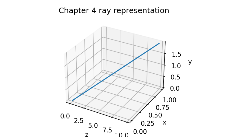
Chapter 5: How a Ray Hits a Curved Surface
A lens drawing makes this step look effortless.
A ray travels forward. It reaches a glass surface. It bends. Then it continues.
In the drawing, the contact point is obvious because your eye sees the line touch the curve. But a program does not see that picture. A program has only numbers:
ray position
ray direction
surface position
surface shape
From those numbers, it must answer a very specific question:
At what point does this ray hit this surface?
This is ray-surface intersection.
It is one of the most important calculations in geometric ray tracing, and it is also one of the easiest to skip in an explanation. Many books and manuals show rays bending at surfaces, then move quickly to Snell’s law. But Snell’s law cannot act until we know where the ray meets the surface and what the surface normal is at that point.
So this chapter slows down.
We will not refract yet. That is Chapter 6. Here, we do only the geometry:
ray + plane  → intersection point
ray + sphere → intersection point
intersection point → aperture check
intersection point → surface normal
By the end of this chapter, a ray will be able to collide with a plane or spherical surface. It will not yet bend. But it will know exactly where bending should happen.
That is a large step.
The problem in one line
From Chapter 4, our ray is:
r(t) = r0 + t d
where:
r0 = ray starting position
d  = normalized ray direction
t  = forward distance parameter
A surface is a set of points satisfying some equation.
For a plane perpendicular to the optical axis:
z = z_v
For a sphere:
(x - cx)² + (y - cy)² + (z - cz)² = R²
Intersection means:
Find the value of
tsuch that the ray pointr(t)lies on the surface.
That is the whole idea.
For a plane, the equation is linear.
For a sphere, the equation becomes quadratic.
For more complex aspheric or freeform surfaces, the equation may need numerical solving. But planes and spheres are enough to build the foundation.
A surface has a vertex
Before writing intersection code, we need one more piece of optical vocabulary.
In a sequential lens prescription, each surface has a vertex position along the optical axis. If the first physical surface is at z = 0, and its thickness is 5 mm, then the next surface vertex is at z = 5 mm.
The vertex is the point where the surface crosses the optical axis.
For a rotationally symmetric spherical surface, we can think of the surface as being placed at a vertex position z_v, with a signed radius R.
Using the convention from earlier chapters:
light generally travels in +z
surface vertex is at z = z_v
signed radius R gives the center of curvature at z = z_v + R
So if:
z_v = 0
R = +50 mm
the sphere center lies at:
z_c = 50 mm
If:
z_v = 5
R = -50 mm
the sphere center lies at:
z_c = -45 mm
This signed-radius convention lets one formula describe both convex and concave surfaces in a sequential optical system.
We will use this model for teaching code.
A small surface class for intersection
The Surface class from earlier chapters stored radius, thickness, material, semi-diameter, and surface type. For intersection, we also need the actual vertex position z.
In a full lens system, we can compute vertex positions from the thickness column. For this chapter, it is helpful to use a separate small class that stores the vertex directly.
from dataclasses import dataclass
from typing import Optional
import math
import numpy as np

@dataclass
class IntersectableSurface:
    radius: float
    z_vertex: float
    semi_diameter: Optional[float] = None
    surface_type: str = "spherical"
    comment: str = ""
This is not meant to replace the prescription data structure permanently. It is a teaching object. It lets us focus on intersection without carrying the whole lens system around.
For example:
front_surface = IntersectableSurface(
    radius=50.0,
    z_vertex=0.0,
    semi_diameter=10.0,
    comment="front spherical surface"
)

image_plane = IntersectableSurface(
    radius=float("inf"),
    z_vertex=50.0,
    semi_diameter=None,
    surface_type="plane",
    comment="image plane"
)
The front surface is spherical. The image plane is a plane at z = 50.
Now we can ask rays to hit them.
Ray-plane intersection
Start with the easiest case.
A plane perpendicular to the optical axis has equation:
z = z_v
The ray is:
r(t) = r0 + t d
If we write only the z coordinate:
z(t) = z0 + t dz
Set it equal to the plane:
z_v = z0 + t dz
Solve for t:
t = (z_v - z0) / dz
This is the same calculation we used in Chapter 4 to propagate to a z plane. Now we will treat it formally as a surface intersection.
def intersect_plane_z(ray, z_plane, eps=1e-12):
    """Return forward distance t where ray intersects plane z = z_plane.

    Returns None if the ray is parallel to the plane or the intersection
    is not in the forward direction.
    """
    dz = ray.direction[2]

    if abs(dz) < eps:
        return None

    t = (z_plane - ray.position[2]) / dz

    if t <= eps:
        return None

    return t
The eps value avoids treating tiny numerical noise as a real forward intersection. In ray tracing, this matters. After a ray has just landed on a surface, we do not want the next intersection test to rediscover the same surface at t = 0.
Test it:
ray = Ray(position=[0, 0, 0], direction=[0.1, 0, 1.0])

t = intersect_plane_z(ray, z_plane=50.0)
p = ray.point_at(t)

print("t =", t)
print("point =", p)
The output should show a point with z = 50. The x value will be nonzero because the ray is tilted.
That is already an intersection.
No drawing was needed.
Turning intersection into an event
We can write a helper that moves the ray to the plane.
def propagate_to_plane(ray, z_plane, refractive_index=1.0):
    t = intersect_plane_z(ray, z_plane)

    if t is None:
        ray.stop(f"missed plane z={z_plane}")
        return ray

    ray.propagate(t, refractive_index=refractive_index)
    return ray
This uses the Ray class from Chapter 4. It updates both position and optical path length.
ray = Ray(position=[0, 0, 0], direction=[0.1, 0, 1.0])
propagate_to_plane(ray, z_plane=50.0)

print(ray.position)
print(ray.opl)
print(ray.alive)
The ray is now sitting on the plane. If this were an image plane, we could record its x and y coordinates as a spot diagram point.
For a plane surface, intersection is easy. The real fun begins with spheres.
Ray-sphere intersection
A spherical optical surface is part of a sphere.
Let its center be:
C = [0, 0, z_c]
and its radius magnitude be:
|R|
A point p = [x, y, z] lies on the sphere if:
||p - C||² = R²
The ray point is:
p(t) = r0 + t d
Substitute the ray into the sphere equation:
||r0 + t d - C||² = R²
This becomes a quadratic equation in t.
Let:
oc = r0 - C
Then:
||oc + t d||² = R²
Expand:
(d · d)t² + 2(d · oc)t + (oc · oc - R²) = 0
So:
a = d · d
b = 2(d · oc)
c = oc · oc - R²
Solve:
t = (-b ± sqrt(b² - 4ac)) / (2a)
Because our ray direction is normalized, a should be 1. But we will compute it anyway. That makes the function more robust.
The discriminant tells us whether the ray hits the sphere:
discriminant = b² - 4ac
If the discriminant is negative, there is no real intersection.
If it is zero, the ray is tangent to the sphere.
If it is positive, the ray intersects the sphere at two mathematical points.
For optical ray tracing, we usually want the nearest positive intersection.
Here is the code:
def sphere_center_from_surface(surface):
    """Return the center of curvature for a spherical surface."""
    if math.isinf(surface.radius):
        return None

    return np.array([0.0, 0.0, surface.z_vertex + surface.radius], dtype=float)

def intersect_sphere(ray, surface, eps=1e-9):
    """Return forward distance t where ray intersects a spherical surface.

    The surface is represented by a vertex position z_vertex and signed radius.
    The sphere center is at z_vertex + radius.
    """
    if math.isinf(surface.radius):
        return intersect_plane_z(ray, surface.z_vertex, eps=eps)

    center = sphere_center_from_surface(surface)
    radius_abs = abs(surface.radius)

    oc = ray.position - center

    a = float(np.dot(ray.direction, ray.direction))
    b = 2.0 * float(np.dot(ray.direction, oc))
    c = float(np.dot(oc, oc) - radius_abs * radius_abs)

    disc = b * b - 4.0 * a * c

    if disc < 0:
        return None

    sqrt_disc = math.sqrt(max(disc, 0.0))

    t1 = (-b - sqrt_disc) / (2.0 * a)
    t2 = (-b + sqrt_disc) / (2.0 * a)

    candidates = [t for t in (t1, t2) if t > eps]

    if not candidates:
        return None

    return min(candidates)
Now test an on-axis ray hitting the first surface of a spherical lens.
surface = IntersectableSurface(
    radius=50.0,
    z_vertex=0.0,
    semi_diameter=10.0,
    comment="front surface"
)

ray = Ray(position=[0.0, 0.0, -20.0], direction=[0.0, 0.0, 1.0])

t = intersect_sphere(ray, surface)
p = ray.point_at(t)

print("t =", t)
print("intersection =", p)
For an on-axis ray, the intersection should be at the vertex:
[0, 0, 0]
or very close to it.
Now try an off-axis parallel ray:
ray = Ray(position=[5.0, 0.0, -20.0], direction=[0.0, 0.0, 1.0])

t = intersect_sphere(ray, surface)
p = ray.point_at(t)

print("t =", t)
print("intersection =", p)
The x coordinate should remain 5, while z should be slightly positive. Why positive? Because a spherical surface with center at z = 50 bulges toward the incoming ray. At height x = 5, the surface point lies slightly to the right of the vertex along z.
This is the sag of the surface appearing naturally from intersection geometry.
Comparing intersection with sag
From Chapter 2, the sag of a spherical surface can be computed as:
sag(r) = R - sign(R) sqrt(R² - r²)
There are several equivalent forms depending on sign convention. For our vertex-and-center convention, the spherical surface satisfies:
x² + y² + (z - (z_v + R))² = R²
Solving for the branch that passes through the vertex gives:
z = z_v + R - sign(R) sqrt(R² - r²)
where:
r² = x² + y²
Let us implement it:
def spherical_sag(x, y, surface):
    """Return z coordinate of a spherical surface at transverse point (x, y)."""
    if math.isinf(surface.radius):
        return surface.z_vertex

    R = surface.radius
    r2 = x*x + y*y
    R2 = R*R

    if r2 > R2:
        return None

    return surface.z_vertex + R - math.copysign(math.sqrt(R2 - r2), R)
Now compare the off-axis intersection:
x, y, z = p
print("intersection z:", z)
print("sag z:", spherical_sag(x, y, surface))
They should match.
This is a good sanity check. The ray-sphere intersection and the surface sag describe the same geometry from two different directions:
intersection: where does this ray meet the surface?
sag: where is the surface at this x, y?
Both are useful.
Why there are two sphere intersections
A line can pass through a sphere in two places.
For a full sphere, this is obvious. The ray enters the sphere on the near side and exits on the far side.
But an optical surface is not the whole sphere. It is a local patch near the vertex. In sequential ray tracing, we normally want the first forward intersection with that surface.
That is why intersect_sphere chooses the smallest positive t.
This works for many teaching examples, but there is a subtle point.
In a real sequential optical system, the expected surface is the next surface in the prescription. The ray may mathematically intersect the far side of the sphere too, but that is not the physical surface patch we mean. Aperture checks and sequential geometry help reject irrelevant intersections.
For ordinary spherical lens surfaces near the optical axis, choosing the nearest positive intersection is the right first rule.
When systems become more complex, robust ray tracing needs additional safeguards:
surface aperture limits
expected propagation direction
local coordinate systems
avoidance of self-intersection
handling of coordinate breaks
surface branch selection
We do not need all of that yet. But it is good to know that professional ray tracers are careful here for a reason.
Aperture check
Finding a mathematical intersection is not enough.
The ray might hit the infinite sphere outside the clear optical area.
A lens surface has a semi-diameter. If the intersection point is too far from the optical axis, the ray is blocked.
For a circular clear aperture:
x² + y² <= semi_diameter²
In code:
def inside_surface_aperture(point, surface):
    """Return True if point is inside the circular clear aperture."""
    if surface.semi_diameter is None:
        return True

    x, y, _ = point
    return x*x + y*y <= surface.semi_diameter * surface.semi_diameter
Test:
surface = IntersectableSurface(
    radius=50.0,
    z_vertex=0.0,
    semi_diameter=10.0
)

points = [
    np.array([0.0, 0.0, 0.0]),
    np.array([5.0, 0.0, 0.0]),
    np.array([10.0, 0.0, 0.0]),
    np.array([11.0, 0.0, 0.0]),
]

for p in points:
    print(p, inside_surface_aperture(p, surface))
The point at x = 11 is outside.
This check may feel mundane. It is not. Aperture clipping affects ray bundles, vignetting, spot diagrams, pupil sampling, illumination, and later image quality calculations.
A ray that hits the mathematical sphere but outside the clear aperture should not continue as though it passed through the lens.
A complete hit record
It is useful to return more than just t.
When a ray hits a surface, we may want:
distance t
intersection point
whether it is inside the aperture
surface normal
surface reference
Let us define a small hit record.
@dataclass
class SurfaceHit:
    t: float
    point: np.ndarray
    normal: np.ndarray
    inside_aperture: bool
    surface: IntersectableSurface
Now we need the normal.
Surface normal for a plane
For a plane z = z_v, a normal can be:
[0, 0, 1]
or:
[0, 0, -1]
Both are geometrically valid. The sign matters for refraction, because Snell’s law uses the normal direction.
For this chapter, we will define a default geometric normal for a plane as:
[0, 0, 1]
Then in Chapter 6, we will orient the normal relative to the incoming ray before applying the vector refraction formula.
def plane_normal():
    return np.array([0.0, 0.0, 1.0])
Surface normal for a sphere
For a sphere, the normal at a point points along the radius from the center to the point.
normal = normalize(point - center)
In code:
def surface_normal(point, surface):
    """Return a geometric unit normal at a point on the surface."""
    if math.isinf(surface.radius) or surface.surface_type == "plane":
        return plane_normal()

    center = sphere_center_from_surface(surface)
    return normalize(point - center)
Test on the vertex of a positive-radius front surface:
surface = IntersectableSurface(radius=50.0, z_vertex=0.0)
point = np.array([0.0, 0.0, 0.0])

print(surface_normal(point, surface))
The normal is:
[0, 0, -1]
Why negative z? Because the sphere center is at z = +50, and the vertex point is at z = 0. The vector from center to vertex points toward negative z.
For the back surface of the same biconvex lens:
back_surface = IntersectableSurface(radius=-50.0, z_vertex=5.0)
point = np.array([0.0, 0.0, 5.0])

print(surface_normal(point, back_surface))
The normal is:
[0, 0, 1]
This is good. The two spherical surfaces have opposite geometric normals at their vertices.
Do not worry yet about whether the normal points “the right way” for refraction. In Chapter 6, we will handle orientation carefully.
For now, the normal is a property of the surface geometry.
The full intersection function
Now combine the pieces.
def intersect_surface(ray, surface, eps=1e-9):
    """Return a SurfaceHit if ray intersects the surface, otherwise None."""
    if surface.surface_type == "plane" or math.isinf(surface.radius):
        t = intersect_plane_z(ray, surface.z_vertex, eps=eps)
    else:
        t = intersect_sphere(ray, surface, eps=eps)

    if t is None:
        return None

    point = ray.point_at(t)
    normal = surface_normal(point, surface)
    inside = inside_surface_aperture(point, surface)

    return SurfaceHit(
        t=t,
        point=point,
        normal=normal,
        inside_aperture=inside,
        surface=surface,
    )
Test it:
surface = IntersectableSurface(
    radius=50.0,
    z_vertex=0.0,
    semi_diameter=10.0,
    comment="front surface"
)

ray = Ray(position=[5.0, 0.0, -20.0], direction=[0.0, 0.0, 1.0])

hit = intersect_surface(ray, surface)

print("t:", hit.t)
print("point:", hit.point)
print("normal:", hit.normal)
print("inside aperture:", hit.inside_aperture)
This is the first time our code has answered the full geometric question.
The ray hit the surface. We know where. We know the normal. We know whether the point is inside the clear aperture.
The next chapter will use the normal and the refractive indices to compute the outgoing ray direction.
Moving the ray to the hit point
A hit record tells us where the ray would hit. But the ray object itself has not moved yet.
We can write:
def propagate_to_surface(ray, surface, refractive_index=1.0):
    """Move a ray to a surface intersection if possible.

    Does not refract. It only propagates to the hit point and checks aperture.
    """
    hit = intersect_surface(ray, surface)

    if hit is None:
        ray.stop(f"missed surface: {surface.comment}")
        return None

    if not hit.inside_aperture:
        ray.propagate(hit.t, refractive_index=refractive_index)
        ray.stop(f"blocked by aperture: {surface.comment}")
        return hit

    ray.propagate(hit.t, refractive_index=refractive_index)

    ray.history.append({
        "event": "surface_hit",
        "surface": surface.comment,
        "point": hit.point.copy(),
        "normal": hit.normal.copy(),
        "inside_aperture": hit.inside_aperture,
    })

    return hit
Try it:
ray = Ray(position=[5.0, 0.0, -20.0], direction=[0.0, 0.0, 1.0])

hit = propagate_to_surface(ray, surface)

print("ray position:", ray.position)
print("ray alive:", ray.alive)
print("stop reason:", ray.stop_reason)
The ray should now sit on the spherical surface.
Again, it has not bent. That restraint is intentional. We want each step to be inspectable.
Chapter 5: where does the ray hit?
Chapter 6: where does it go after hitting?
Do not mix those too early.
Visualizing ray-sphere hits
A picture helps, as long as we remember that the picture is derived from the computation.
Let us trace several parallel rays into a spherical surface and plot their hit points.
import matplotlib.pyplot as plt

surface = IntersectableSurface(
    radius=50.0,
    z_vertex=0.0,
    semi_diameter=10.0,
    comment="front spherical surface"
)

rays = [
    Ray(position=[x, 0.0, -20.0], direction=[0.0, 0.0, 1.0])
    for x in np.linspace(-9.0, 9.0, 7)
]

hit_points = []

for ray in rays:
    hit = intersect_surface(ray, surface)
    if hit is not None and hit.inside_aperture:
        hit_points.append(hit.point)

hit_points = np.array(hit_points)

# Draw surface profile in x-z plane.
xs = np.linspace(-10.0, 10.0, 300)
zs = [spherical_sag(x, 0.0, surface) for x in xs]

plt.plot(zs, xs, label="spherical surface")

# Draw incoming ray segments and hit points.
for ray, hp in zip(rays, hit_points):
    plt.plot([ray.position[2], hp[2]], [ray.position[0], hp[0]], linewidth=0.8)

plt.scatter(hit_points[:, 2], hit_points[:, 0], label="hit points")
plt.xlabel("z [mm]")
plt.ylabel("x [mm]")
plt.title("Parallel rays hitting a spherical surface")
plt.gca().set_aspect("equal", adjustable="box")
plt.legend()
plt.show()
This plot should show straight parallel rays reaching different points on the curved surface. The off-axis rays hit the surface at different z positions because the surface is curved.
This is not merely a drawing. Every contact point was computed.
That distinction is the point of the chapter.
What if the ray misses?
A ray may miss a sphere.
For example, if the ray travels far outside the surface:
ray = Ray(position=[100.0, 0.0, -20.0], direction=[0.0, 0.0, 1.0])
hit = intersect_surface(ray, surface)

print(hit)
This may return None, or it may mathematically hit the large parent sphere depending on geometry. But it should fail the aperture check if the surface semi-diameter is small.
That is why both checks matter:
Does the ray intersect the mathematical surface?
Is the intersection inside the clear aperture?
For optical surfaces, the second question is often just as important as the first.
A ray can hit the sphere but miss the lens.
Tangent rays and numerical precision
If a ray just grazes a sphere, the quadratic discriminant is close to zero. Numerically, this can be delicate.
In exact math:
discriminant = 0
means tangent.
In floating-point computation, a value that should be zero might appear as:
-1e-14
because of rounding.
That is why some ray tracers use tolerances. A robust function may treat very small negative discriminants as zero.
We used:
sqrt_disc = math.sqrt(max(disc, 0.0))
but only after checking:
if disc < 0:
    return None
For teaching code, this is acceptable. For more robust code, we might write:
if disc < -eps:
    return None
disc = max(disc, 0.0)
This would allow tiny negative values caused by numerical roundoff.
Here is a more tolerant version:
def intersect_sphere_tolerant(ray, surface, eps=1e-9):
    if math.isinf(surface.radius):
        return intersect_plane_z(ray, surface.z_vertex, eps=eps)

    center = sphere_center_from_surface(surface)
    radius_abs = abs(surface.radius)
    oc = ray.position - center

    a = float(np.dot(ray.direction, ray.direction))
    b = 2.0 * float(np.dot(ray.direction, oc))
    c = float(np.dot(oc, oc) - radius_abs * radius_abs)

    disc = b*b - 4.0*a*c

    if disc < -eps:
        return None

    disc = max(disc, 0.0)
    sqrt_disc = math.sqrt(disc)

    t1 = (-b - sqrt_disc) / (2.0*a)
    t2 = (-b + sqrt_disc) / (2.0*a)

    candidates = [t for t in (t1, t2) if t > eps]

    if not candidates:
        return None

    return min(candidates)
Numerical tolerance is not an advanced luxury. It is part of making geometry work on finite-precision machines.
Intersections and local coordinates
So far, all surfaces are centered on the z axis. That is enough for early chapters.
A real optical design program needs local coordinates. A surface may be tilted, decentered, or placed after a coordinate break. The ray may need to be transformed into the surface’s local coordinate system, intersected there, and transformed back.
The general pattern is:
global ray
→ transform into local surface coordinates
→ compute intersection
→ compute local normal
→ transform point and normal back to global coordinates
This sounds like a complication, and it is. But notice that the basic intersection problem remains the same. The local coordinate system is there to make the surface equation simpler.
We will not implement coordinate breaks in this book’s core teaching code. That would distract from the main computation chain. But when you see a professional library handling tilted mirrors, prisms, off-axis systems, or freeform surfaces, remember that it is doing this kind of coordinate bookkeeping.
The skeleton is still:
ray + surface equation → t → point → normal
The coordinate transforms just prepare the inputs and return the result to the global system.
Building surface vertices from a prescription
In Chapter 2, a lens prescription gave us thicknesses. For intersection, we need surface vertex positions.
Let us write a helper that converts a sequence of prescription surfaces into intersectable surfaces with z positions.
Assume we have a Surface class like before:
@dataclass
class Surface:
    radius: float
    thickness: float
    material_after: str = "air"
    semi_diameter: Optional[float] = None
    conic: float = 0.0
    is_stop: bool = False
    surface_type: str = "spherical"
    comment: str = ""
Now convert:
def build_intersectable_surfaces(prescription_surfaces):
    """Convert prescription surfaces into surfaces with vertex z positions.

    Skips an object-at-infinity row if present.
    """
    surfaces = prescription_surfaces

    if surfaces and math.isinf(surfaces[0].thickness):
        surfaces = surfaces[1:]

    z = 0.0
    result = []

    for s in surfaces:
        surface_type = s.surface_type

        if math.isinf(s.radius):
            surface_type = "plane"

        result.append(IntersectableSurface(
            radius=s.radius,
            z_vertex=z,
            semi_diameter=s.semi_diameter,
            surface_type=surface_type,
            comment=s.comment,
        ))

        if not math.isinf(s.thickness):
            z += s.thickness

    return result
Now a lens prescription can feed intersection code.
This is the first time the data structure from Chapter 2 starts to move real rays from Chapter 4.
The chain is becoming executable:
prescription thicknesses
→ surface vertex positions
→ ray-surface intersections
→ hit points and normals
A no-refraction trace through two surfaces
Let us trace a ray to the two surfaces of a singlet, but without bending it.
This is physically wrong as optics, but useful as geometry.
prescription = [
    Surface(
        radius=float("inf"),
        thickness=float("inf"),
        surface_type="object",
        comment="object at infinity"
    ),
    Surface(
        radius=50.0,
        thickness=5.0,
        material_after="N-BK7",
        semi_diameter=10.0,
        comment="front surface"
    ),
    Surface(
        radius=-50.0,
        thickness=45.0,
        material_after="air",
        semi_diameter=10.0,
        comment="back surface"
    ),
    Surface(
        radius=float("inf"),
        thickness=0.0,
        surface_type="image",
        comment="image plane"
    ),
]

surfaces = build_intersectable_surfaces(prescription)

ray = Ray(position=[3.0, 0.0, -20.0], direction=[0.0, 0.0, 1.0])

for s in surfaces:
    hit = propagate_to_surface(ray, s, refractive_index=1.0)

    if hit is None or not ray.alive:
        break

    print(s.comment, ray.position, "normal", hit.normal)
The ray passes through the front surface, then the back surface, then reaches the image plane. It does not bend, so it is not a real optical trace. But it confirms that the geometry is working.
This kind of intermediate test is extremely useful.
Before adding refraction, make sure intersections work.
Before adding wavefronts, make sure refraction works.
Before adding PSF, make sure OPD works.
A black box is often just too many untested steps stacked together.
The image plane is just another plane intersection
The image plane is often special in interpretation, but geometrically it is simple.
It is usually represented as a plane perpendicular to the optical axis:
z = z_image
When rays reach it, we record their transverse coordinates:
x_image, y_image
Those coordinates become spot diagram points.
The image plane does not need refraction if it is only an evaluation surface. It is where we measure the ray, not necessarily a physical boundary.
That is why our build_intersectable_surfaces function can treat an infinite-radius image surface as a plane.
Later, in a full trace, the image plane will be the last surface. Rays that reach it contribute to geometric image analysis.
Surface normal and refraction are separate jobs
It is tempting to jump straight from intersection to bending. Let us resist that for one more section.
At a surface hit, we now know:
point
normal
material before
material after
ray direction
wavelength
The refraction calculation will use:
incoming direction
surface normal
n_before
n_after
But the normal itself is a geometric object. It should be computed before and independently from Snell’s law.
This separation keeps the code clean:
intersection code:
    returns point and normal

material code:
    returns n_before and n_after

refraction code:
    returns new direction
If all of that is mixed into one function, debugging becomes painful.
When a ray bends incorrectly, you will not know whether the point was wrong, the normal was wrong, the refractive index was wrong, or the vector formula was wrong.
Small functions are not just stylistic preference. They make optical errors visible.
A preview of the next step
At the end of this chapter, a ray hitting a spherical surface has an incoming direction and a normal.
For example:
ray = Ray(position=[5.0, 0.0, -20.0], direction=[0.0, 0.0, 1.0])
surface = IntersectableSurface(radius=50.0, z_vertex=0.0, semi_diameter=10.0)

hit = intersect_surface(ray, surface)

print("incoming direction:", ray.direction)
print("surface normal:", hit.normal)
The incoming direction might be:
[0, 0, 1]
The normal will be tilted because the ray hit the curved surface away from the axis:
normal ≈ [small x component, 0, mostly negative z]
That tilted normal is exactly why an off-axis ray bends differently from an on-axis ray. Snell’s law does not see the whole lens drawing. It sees the local surface normal at the hit point.
This is the local nature of refraction.
A curved lens is not magic. It is many local surface normals changing from point to point.
That is a beautiful thought, and also a computationally useful one.
Common mistakes in ray-surface intersection
Let us name the traps before they bite.
Mistake 1: Forgetting to choose the forward intersection
The quadratic equation gives mathematical roots. Some may lie behind the ray. Use positive t values and choose the nearest valid one.
Mistake 2: Ignoring aperture limits
A ray can intersect the parent sphere but outside the actual lens surface. Always check the clear aperture.
Mistake 3: Confusing radius sign with radius magnitude
The signed radius locates the center of curvature. The sphere equation uses the magnitude of the radius.
center z = z_vertex + R
sphere radius = |R|
Mistake 4: Using the wrong surface branch
A full sphere has two sides. A sequential optical surface is a local patch near its vertex. In ordinary cases, the nearest positive intersection works, but more complex systems require care.
Mistake 5: Not using tolerances
Floating-point calculations are not exact. Very small negative discriminants or tiny t values can cause false misses or self-intersections.
Mistake 6: Mixing sag and intersection logic
Sag gives surface height for a known transverse coordinate. Intersection solves where a ray meets the surface. They are related, but they answer different questions.
Mistake 7: Computing refraction before verifying the hit
Do not refract a ray that missed the surface or was blocked by the aperture.
Mistake 8: Losing the normal direction
The surface normal must be normalized and stored carefully. The refraction chapter will need it.
What this chapter gives us
We now have the geometric core of ray tracing.
We can:
represent a plane surface
represent a spherical surface with signed radius
compute ray-plane intersection
compute ray-sphere intersection
choose the nearest forward hit
check whether the hit is inside the clear aperture
compute the surface normal at the hit point
move the ray to the surface
record the hit
This is not a small accomplishment.
A ray in Chapter 4 could only travel through empty space.
A ray after Chapter 5 can find the glass.
It still cannot bend. But that is now the only missing action for a basic real ray trace.
The next chapter will add it.
We will take the incoming direction, the surface normal, and the refractive indices from Chapter 3. Then we will compute the outgoing direction using Snell’s law in vector form.
That is the moment the ray will finally do what the drawing has always shown:
it will hit the surface
and change direction
But this time, we will know exactly where that happened, which normal was used, which indices were used, and how the new direction was calculated.
That is how a software command becomes a calculation you can inspect.
Generated validation figure
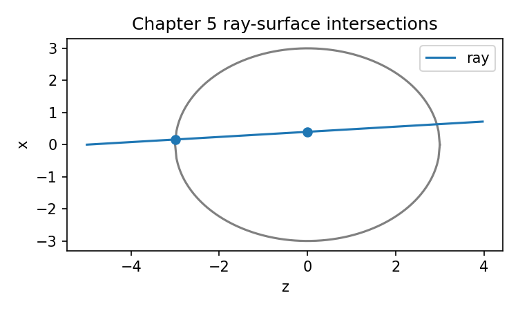
Chapter 6: How Refraction Direction Is Computed
A ray has now reached the surface.
That sentence sounds simple only because we have already done the hidden work.
In Chapter 4, we gave the ray a position, a direction, a wavelength, an intensity, and an optical path length. In Chapter 5, we made that ray collide with a plane or spherical surface. We computed the hit point. We checked the clear aperture. We computed the local surface normal.
Now the ray is sitting at the surface.
It has an incoming direction:
d_in
The surface has a local normal:
N
The material model gives refractive indices on the two sides:
n1 = refractive index before the surface
n2 = refractive index after the surface
The next question is the one every optics student expects:
In what direction does the ray go after refraction?
This chapter answers that question.
We will begin with scalar Snell’s law, but we will not stay there. Optical software does not usually trace rays by drawing angles with a protractor. It has direction vectors and surface normals. So the useful form is vector refraction.
That is where many errors happen.
The formula itself is not very long. The hard parts are:
normal direction
unit vectors
which index is n1 and which is n2
total internal reflection
numerical tolerance
We will go slowly. This is one of the load-bearing chapters of the book.
After this chapter, the ray will finally do what lens drawings have shown all along:
hit a surface
bend according to the local normal and refractive indices
continue in a new direction
Only now, the bending will be computed.
Start with scalar Snell’s law
The familiar form of Snell’s law is:
n1 sin θ1 = n2 sin θ2
where:
n1 = refractive index of the incident medium
n2 = refractive index of the transmitted medium
θ1 = incident angle measured from the surface normal
θ2 = refracted angle measured from the surface normal
This law says that the ray changes direction when it crosses between media with different refractive indices.
If light goes from air into glass:
n1 ≈ 1.0
n2 ≈ 1.5
then the ray bends toward the normal.
If light goes from glass into air:
n1 ≈ 1.5
n2 ≈ 1.0
then the ray bends away from the normal.
At normal incidence, where θ1 = 0, the ray does not change direction. It may change speed and wavelength inside the medium, but its geometric direction remains the same.
Let us first write a scalar angle function, just to see the law numerically.
import math

def snell_angle(theta1_deg, n1, n2):
    """Return refracted angle in degrees using scalar Snell's law.

    theta1_deg is measured from the surface normal.
    Returns None if total internal reflection occurs.
    """
    theta1 = math.radians(theta1_deg)
    sin_theta2 = (n1 / n2) * math.sin(theta1)

    if abs(sin_theta2) > 1.0:
        return None

    theta2 = math.asin(sin_theta2)
    return math.degrees(theta2)
Try air to glass:
for theta in [0, 10, 20, 30, 40]:
    theta2 = snell_angle(theta, n1=1.0, n2=1.5)
    print(theta, "→", theta2)
The refracted angles are smaller. The ray bends toward the normal.
Try glass to air:
for theta in [0, 10, 20, 30, 40, 50]:
theta2 = snell_angle(theta, n1=1.5, n2=1.0)
print(theta, "→", theta2)
At some incident angle, the function returns None. That is total internal reflection.
The scalar form is useful for intuition. But it is not enough for real ray tracing.
A ray tracer does not usually store “angle from normal.” It stores:
incoming direction vector
surface normal vector
So we need the vector version.
Why scalar angles are not enough
Imagine a ray hitting a spherical surface away from the optical axis.
The local normal is not [0, 0, 1]. It points outward from the sphere center through the hit point. Its x and y components may be nonzero.
In scalar Snell’s law, you can say:
the incident angle is θ1
the refracted angle is θ2
But in three-dimensional code, that does not tell you the outgoing vector. There are infinitely many directions that make the same angle with a normal unless you also know the plane of incidence.
The plane of incidence is defined by:
incoming direction
surface normal
The refracted ray must stay in that plane. A vector formula handles this automatically.
So the computational task is:
given:
d_in, normal, n1, n2
compute:
d_out
where both direction vectors are unit length.
That is the function we want:
d_out = refract_direction(d_in, normal, n1, n2)
But before writing it, we must handle a surprisingly important detail.
The normal has two possible directions
A surface normal can point in either of two opposite directions.
For a plane, both of these are valid normals:
[0, 0, 1]
[0, 0, -1]
For a sphere, the geometric normal often points outward from the sphere center. That is a perfectly good geometric normal. But for refraction, the formula needs the normal to be oriented consistently relative to the incoming ray.
This is where many ray tracers first go wrong.
Let us define a convention:
Before applying the vector refraction formula, orient the normal so that it points against the incoming ray.
In other words, after orientation:
dot(d_in, normal) <= 0
If the incoming ray points roughly in +z, the oriented normal should point roughly back toward the incident side.
Here is the helper function:
import numpy as np
def normalize(v):
"""Return a unit-length copy of vector v."""
v = np.asarray(v, dtype=float)
norm = np.linalg.norm(v)
if norm == 0:
raise ValueError("Cannot normalize a zero vector.")
return v / norm
def orient_normal_against_ray(direction, normal):
"""Orient normal so that it points against the incoming direction."""
d = normalize(direction)
n = normalize(normal)
if np.dot(d, n) > 0:
n = -n
return n
Test it:
d_in = np.array([0.0, 0.0, 1.0])
print(orient_normal_against_ray(d_in, [0, 0, 1]))
print(orient_normal_against_ray(d_in, [0, 0, -1]))
Both cases should produce:
[ 0. 0. -1.]
That is what we want. The refraction function should not care whether the surface gave us [0,0,1] or [0,0,-1]. It should orient the normal before using it.
This small function removes a large class of sign bugs.
The vector refraction formula
Let:
i = incoming unit direction
n = unit normal oriented against the incoming ray
η = n1 / n2
The cosine of the incident angle is:
cosθ1 = - i · n
The transmitted direction can be written as:
t = η i + (η cosθ1 - cosθ2) n
where:
cosθ2 = sqrt(1 - η²(1 - cos²θ1))
The term under the square root is important:
k = 1 - η²(1 - cos²θ1)
If k < 0, there is no real refracted ray. That is total internal reflection.
This is the complete computational logic.
normalize incoming direction
normalize and orient normal
compute η = n1 / n2
compute cosθ1
compute k
if k < 0: total internal reflection
else compute outgoing direction
normalize outgoing direction
Now write it in Python.
def refract_direction(direction, normal, n1, n2, eps=1e-12):
"""Compute refracted ray direction using vector Snell's law.
Parameters
----------
direction:
Incoming ray direction. It does not need to be pre-normalized.
normal:
Surface normal at the hit point. It may point either way;
this function orients it against the incoming ray.
n1:
Refractive index of the incident medium.
n2:
Refractive index of the transmitted medium.
Returns
-------
A unit outgoing direction vector, or None if total internal reflection occurs.
"""
i = normalize(direction)
n = orient_normal_against_ray(i, normal)
eta = n1 / n2
cos_theta1 = -float(np.dot(i, n))
# Numerical safety: keep cosine inside valid range.
cos_theta1 = max(-1.0, min(1.0, cos_theta1))
sin2_theta2 = eta * eta * (1.0 - cos_theta1 * cos_theta1)
if sin2_theta2 > 1.0 + eps:
return None
# Clamp tiny numerical overshoot.
sin2_theta2 = min(1.0, max(0.0, sin2_theta2))
cos_theta2 = math.sqrt(1.0 - sin2_theta2)
t = eta * i + (eta * cos_theta1 - cos_theta2) * n
return normalize(t)
This function is the heart of the chapter.
It is not a black box. It is a direct computational form of Snell’s law.
The incoming ray direction and the surface normal define the plane of incidence. The refractive-index ratio controls the bending. The square root test detects total internal reflection.
Now we must test it carefully.
A helper for measuring angles
To compare with scalar Snell’s law, we need a way to measure the angle between a direction and the normal line.
The normal line has two directions, normal and -normal, so we use the absolute value of the dot product.
def angle_to_normal_line(direction, normal):
"""Return the smaller angle between a direction and the normal line."""
d = normalize(direction)
n = normalize(normal)
c = abs(float(np.dot(d, n)))
c = max(-1.0, min(1.0, c))
return math.degrees(math.acos(c))
Now we can test vector refraction against scalar Snell’s law.
Test 1: normal incidence
A ray traveling along the normal should not change direction.
d_in = np.array([0.0, 0.0, 1.0])
normal = np.array([0.0, 0.0, -1.0])
d_out = refract_direction(d_in, normal, n1=1.0, n2=1.5)
print("incoming:", d_in)
print("outgoing:", d_out)
print("angle:", angle_to_normal_line(d_out, normal))
The outgoing direction should still be:
[0, 0, 1]
The angle to the normal line should be 0.
This is a basic sanity check. If this fails, do not continue. Fix the normal orientation or formula first.
Test 2: air to glass
Now use a ray 30 degrees from the normal. Let the normal line be the z axis, and let the ray travel in the x-z plane.
def direction_from_angle_to_z(theta_deg):
"""Direction in x-z plane, traveling generally in +z."""
theta = math.radians(theta_deg)
return normalize([math.sin(theta), 0.0, math.cos(theta)])
d_in = direction_from_angle_to_z(30.0)
normal = np.array([0.0, 0.0, -1.0])
d_out = refract_direction(d_in, normal, n1=1.0, n2=1.5)
print("incoming angle:", angle_to_normal_line(d_in, normal))
print("outgoing angle:", angle_to_normal_line(d_out, normal))
print("scalar Snell:", snell_angle(30.0, n1=1.0, n2=1.5))
print("outgoing direction:", d_out)
The vector outgoing angle should match scalar Snell’s law.
Air to glass bends toward the normal, so the outgoing angle should be smaller than 30 degrees.
This test confirms that the vector formula and scalar law agree in a simple plane case.
Test 3: glass to air
Now reverse the indices.
d_in = direction_from_angle_to_z(30.0)
normal = np.array([0.0, 0.0, -1.0])
d_out = refract_direction(d_in, normal, n1=1.5, n2=1.0)
print("incoming angle:", angle_to_normal_line(d_in, normal))
print("outgoing angle:", angle_to_normal_line(d_out, normal))
print("scalar Snell:", snell_angle(30.0, n1=1.5, n2=1.0))
print("outgoing direction:", d_out)
Glass to air bends away from the normal, so the outgoing angle should be larger than 30 degrees.
Again, the vector and scalar results should match.
Test 4: total internal reflection
Total internal reflection occurs when light tries to pass from a higher-index medium to a lower-index medium at too steep an angle.
The critical angle satisfies:
sin θc = n2 / n1
for n1 > n2.
For glass to air:
θc = arcsin(1.0 / 1.5) ≈ 41.8 degrees
So a 50-degree incident angle should not produce a transmitted ray.
d_in = direction_from_angle_to_z(50.0)
normal = np.array([0.0, 0.0, -1.0])
d_out = refract_direction(d_in, normal, n1=1.5, n2=1.0)
print(d_out)
The result should be:
None
That does not mean the ray disappears physically. It means there is no refracted transmitted ray. The interface would reflect the ray internally. In a refractive lens tracing path, we may stop the ray or handle reflection depending on the system model.
For this book’s basic refractive ray tracer, we will stop the ray and record the reason.
Total internal reflection is not an error
It is tempting to treat None as a failure of the code. It is not.
Total internal reflection is a real physical condition. The code is doing its job by detecting that no refracted direction exists.
What the ray tracer does next depends on the optical model.
For a purely refractive system, it may mark the ray invalid:
stop ray: total internal reflection
For a system that supports reflection, it may compute a reflected direction instead:
d_reflect = d_in - 2(d_in · n)n
We will not build a reflective ray tracer here. But it is useful to know that total internal reflection is a branching event, not a numerical accident.
In our basic lens ray tracer, stopping the ray is the right first behavior.
A function for reflection, for comparison
Even though this chapter focuses on refraction, reflection is short enough to show. It also helps clarify normal orientation.
def reflect_direction(direction, normal):
"""Reflect direction across a surface normal."""
i = normalize(direction)
n = normalize(normal)
return normalize(i - 2.0 * np.dot(i, n) * n)
If total internal reflection occurs, a more complete tracer could use this. For now, we will simply stop refractive rays when refraction is impossible.
The main chain of this book is lens imaging, not mirror systems.
Putting wavelength back into the calculation
So far, we have used fixed values like:
n1 = 1.0
n2 = 1.5
But in Chapter 3, we already learned that a real material gives:
n = n(λ)
The ray carries wavelength:
ray.wavelength_um
So at each surface, the tracing code should ask the material library:
n1 = materials.n(material_before, ray.wavelength_um)
n2 = materials.n(material_after, ray.wavelength_um)
That is how chromatic refraction enters the ray tracer.
A blue ray and a red ray may have the same incoming direction and hit the same surface point. But because the glass has different refractive index at different wavelengths, their outgoing directions will differ slightly.
Let us demonstrate this with a plane interface.
Assume we have an N-BK7 material model from Chapter 3:
# N_BK7.n(wavelength_um) returns refractive index.
# For this example, assume N_BK7 is already defined.
Now compare blue, green, and red rays entering glass at 30 degrees.
F_LINE_UM = 0.4861327
D_LINE_UM = 0.5875618
C_LINE_UM = 0.6562725
normal = np.array([0.0, 0.0, -1.0])
d_in = direction_from_angle_to_z(30.0)
for wl in [F_LINE_UM, D_LINE_UM, C_LINE_UM]:
n_glass = N_BK7.n(wl)
d_out = refract_direction(d_in, normal, n1=1.0, n2=n_glass)
angle = angle_to_normal_line(d_out, normal)
print(f"{wl:.7f} µm n={n_glass:.7f} outgoing angle={angle:.6f} deg")
The differences will be small. But they are real.
Shorter wavelengths usually see a higher refractive index in normal dispersion, so the blue ray bends slightly more toward the normal than the red ray.
That is chromatic behavior entering through one line of code:
n_glass = N_BK7.n(wl)
This is why Chapter 3 was not optional. Without wavelength-dependent material indices, a ray tracer cannot show chromatic aberration.
Refraction at a curved surface
Now let us use what Chapter 5 gave us: a hit point and a local normal on a spherical surface.
Imagine a parallel ray entering the front surface of a spherical N-BK7 lens.
We already have:
ray
surface
intersect_surface(ray, surface)
The hit record contains:
hit.point
hit.normal
Now we compute the outgoing direction.
surface = IntersectableSurface(
radius=50.0,
z_vertex=0.0,
semi_diameter=10.0,
comment="front spherical surface"
)
ray = Ray(
position=[5.0, 0.0, -20.0],
direction=[0.0, 0.0, 1.0],
wavelength_um=0.5875618
)
hit = intersect_surface(ray, surface)
n_air = 1.0
n_glass = N_BK7.n(ray.wavelength_um)
d_out = refract_direction(
direction=ray.direction,
normal=hit.normal,
n1=n_air,
n2=n_glass
)
print("hit point:", hit.point)
print("surface normal:", hit.normal)
print("incoming direction:", ray.direction)
print("outgoing direction:", d_out)
For an off-axis ray, the surface normal has an x component. The outgoing direction will also gain an x component. That is the surface focusing the ray.
This is the local reason a lens works.
A lens does not “know” where the image plane is. At each surface, the ray only sees:
local normal
incoming direction
index before
index after
The global focusing behavior emerges from many local refractions and propagations.
That is a powerful idea. It is also exactly what ray-tracing software computes.
Updating the ray at the surface
A refraction function returns a direction. But our ray object must actually be updated.
A surface interaction has several steps:
1. find the surface hit
2. propagate the ray to the hit point through the current medium
3. check aperture
4. compute refractive indices
5. compute refracted direction
6. update the ray direction
7. continue into the next medium
Chapters 3, 4, and 5 gave us almost all pieces. Now we combine them.
First, define a small result object:
from dataclasses import dataclass
@dataclass
class RefractionResult:
success: bool
direction: np.ndarray | None
reason: str = ""
If your Python version does not support np.ndarray | None, use Optional[np.ndarray] from typing.
Now wrap the refraction call:
def refract_at_surface(ray, hit, n1, n2):
"""Return a refraction result for a ray at a surface hit."""
d_out = refract_direction(
direction=ray.direction,
normal=hit.normal,
n1=n1,
n2=n2
)
if d_out is None:
return RefractionResult(
success=False,
direction=None,
reason="total internal reflection"
)
return RefractionResult(
success=True,
direction=d_out,
reason=""
)
Then a surface interaction can update the ray:
def interact_refractive_surface(ray, surface, n1, n2):
"""Propagate ray to a surface and refract it.
This function assumes n1 is the index of the medium before the surface
and n2 is the index after the surface.
"""
if not ray.alive:
return None
hit = intersect_surface(ray, surface)
if hit is None:
ray.stop(f"missed surface: {surface.comment}")
return None
# Propagate through the incident medium to the hit point.
ray.propagate(hit.t, refractive_index=n1)
if not hit.inside_aperture:
ray.stop(f"blocked by aperture: {surface.comment}")
return hit
result = refract_at_surface(ray, hit, n1=n1, n2=n2)
if not result.success:
ray.stop(result.reason)
return hit
old_direction = ray.direction.copy()
ray.direction = result.direction
ray.history.append({
"event": "refract",
"surface": surface.comment,
"point": ray.position.copy(),
"normal": hit.normal.copy(),
"n1": n1,
"n2": n2,
"direction_before": old_direction,
"direction_after": ray.direction.copy(),
})
return hit
This function is a milestone.
A ray can now:
find a surface
move to the surface
check aperture
bend into the next medium
carry on with a new direction
That is real ray tracing.
Still simple, yes. But real.
Tracing through a single spherical interface
Let us trace a few parallel rays entering a spherical air-to-glass interface.
surface = IntersectableSurface(
radius=50.0,
z_vertex=0.0,
semi_diameter=10.0,
comment="air-to-glass spherical surface"
)
rays = [
Ray(position=[x, 0.0, -20.0], direction=[0.0, 0.0, 1.0], wavelength_um=0.5875618)
for x in np.linspace(-8.0, 8.0, 5)
]
n_air = 1.0
n_glass = N_BK7.n(0.5875618)
for ray in rays:
interact_refractive_surface(ray, surface, n1=n_air, n2=n_glass)
print(
"position:", ray.position,
"direction:", ray.direction,
"alive:", ray.alive
)
The on-axis ray should remain along the z direction. Off-axis rays should bend inward. Rays on opposite sides should bend symmetrically.
This symmetry is a useful sanity check. If both off-axis rays bend in the same transverse direction, something is wrong.
Most likely causes:
normal sign error
surface center sign error
wrong n1/n2 order
incorrect intersection branch
The debugging trail is already clear because we kept the functions separate.
Visualizing the bend
Let us plot incoming and outgoing segments around the spherical surface.
import matplotlib.pyplot as plt
def line_points(start, direction, length):
start = np.asarray(start, dtype=float)
direction = normalize(direction)
end = start + length * direction
return start, end
surface = IntersectableSurface(
radius=50.0,
z_vertex=0.0,
semi_diameter=10.0,
comment="front spherical surface"
)
rays = [
Ray(position=[x, 0.0, -20.0], direction=[0.0, 0.0, 1.0], wavelength_um=0.5875618)
for x in np.linspace(-8.0, 8.0, 7)
]
plt.figure()
# Draw surface profile in x-z plane.
xs = np.linspace(-10.0, 10.0, 300)
zs = [spherical_sag(x, 0.0, surface) for x in xs]
plt.plot(zs, xs, label="spherical surface")
for ray in rays:
start = ray.position.copy()
incoming_dir = ray.direction.copy()
hit = interact_refractive_surface(ray, surface, n1=1.0, n2=N_BK7.n(ray.wavelength_um))
if hit is None:
continue
hit_point = ray.position.copy()
outgoing_dir = ray.direction.copy()
# Incoming segment.
plt.plot([start[2], hit_point[2]], [start[0], hit_point[0]], linewidth=0.8)
# Outgoing segment preview.
end = hit_point + 25.0 * outgoing_dir
plt.plot([hit_point[2], end[2]], [hit_point[0], end[0]], linewidth=0.8)
plt.xlabel("z [mm]")
plt.ylabel("x [mm]")
plt.title("Refraction at a spherical air-glass surface")
plt.gca().set_aspect("equal", adjustable="box")
plt.legend()
plt.show()
The drawing is now earned.
It is not a decorative sketch. It is a visualization of computed intersections and computed refracted directions.
This is exactly the kind of shift we want throughout the book.
The order of n1 and n2 matters
At the front surface of a lens:
air → glass
so:
n1 = n_air
n2 = n_glass
At the back surface:
glass → air
so:
n1 = n_glass
n2 = n_air
If you reverse them, the ray will bend the wrong way.
This is why the material transition logic from Chapter 3 matters. The tracing code should not guess.
A function like this is helpful:
def material_before_after(lens, surface_index, starting_material="air"):
"""Return material names before and after a sequential surface."""
if surface_index == 0:
before = starting_material
else:
before = lens.surfaces[surface_index - 1].material_after
after = lens.surfaces[surface_index].material_after
return before, after
def index_transition(lens, materials, surface_index, wavelength_um):
before_name, after_name = material_before_after(lens, surface_index)
n_before = materials.n(before_name, wavelength_um)
n_after = materials.n(after_name, wavelength_um)
return n_before, n_after
Then at a surface:
n1, n2 = index_transition(lens, materials, surface_index, ray.wavelength_um)
That one line encodes the correct refractive-index order.
Without this discipline, multi-surface tracing becomes fragile.
Combining intersection and material transition
In a sequential system, a full surface step needs both geometry and material data.
The surface geometry tells us:
where the ray hits
what the normal is
whether the ray is inside the aperture
The prescription and material library tell us:
n_before
n_after
The refraction formula tells us:
new direction
Let us sketch the combined loop.
def trace_refractive_surfaces(ray, intersectable_surfaces, lens, materials, start_index=1):
"""Trace one ray through refractive surfaces.
This is a simplified skeleton. It assumes intersectable_surfaces and
lens.surfaces correspond to the same sequential surfaces after object row handling.
"""
for local_i, surface in enumerate(intersectable_surfaces):
if not ray.alive:
break
# Skip object-like surfaces if present.
if surface.comment.lower().startswith("object"):
continue
# Image plane is an evaluation surface, not a refracting boundary.
if surface.comment.lower().startswith("image"):
hit = intersect_surface(ray, surface)
if hit is None:
ray.stop("missed image plane")
break
ray.propagate(hit.t, refractive_index=1.0)
break
prescription_index = start_index + local_i
n1, n2 = index_transition(
lens,
materials,
prescription_index,
ray.wavelength_um
)
interact_refractive_surface(ray, surface, n1=n1, n2=n2)
return ray
This is still simplified. It assumes a straightforward sequential system. It does not handle coordinate breaks, mirrors, reflective coatings, immersion media, tilted surfaces, or advanced aperture definitions.
That is fine.
Here is the computational chain in one place:
ray wavelength
→ material indices
→ surface hit
→ normal
→ vector Snell refraction
→ updated ray direction
That is the core of real ray tracing.
A two-surface singlet trace
Now let us make a basic biconvex singlet.
We will trace rays through:
front surface: air → N-BK7
back surface: N-BK7 → air
image plane: evaluation only
Use the surfaces from earlier chapters:
front = IntersectableSurface(
radius=50.0,
z_vertex=0.0,
semi_diameter=10.0,
comment="front surface"
)
back = IntersectableSurface(
radius=-50.0,
z_vertex=5.0,
semi_diameter=10.0,
comment="back surface"
)
image = IntersectableSurface(
radius=float("inf"),
z_vertex=50.0,
semi_diameter=None,
surface_type="plane",
comment="image plane"
)
Trace one ray:
ray = Ray(
position=[5.0, 0.0, -20.0],
direction=[0.0, 0.0, 1.0],
wavelength_um=0.5875618
)
n_air = 1.0
n_glass = N_BK7.n(ray.wavelength_um)
interact_refractive_surface(ray, front, n1=n_air, n2=n_glass)
interact_refractive_surface(ray, back, n1=n_glass, n2=n_air)
# Propagate to image plane in air.
hit_image = intersect_surface(ray, image)
ray.propagate(hit_image.t, refractive_index=n_air)
print("image point:", ray.position)
print("final direction:", ray.direction)
print("OPL:", ray.opl)
print("alive:", ray.alive)
print("stop reason:", ray.stop_reason)
This is the first complete refractive trace through a simple lens.
It is not yet a polished optical design program. It does not aim rays from a proper object field. It does not compute best focus. It does not manage all edge cases. But it performs the essential operations:
air propagation
front surface intersection
air-to-glass refraction
glass propagation
back surface intersection
glass-to-air refraction
air propagation to image plane
That is the skeleton under many optical design tools.
From one ray to a small fan
Let us trace a fan of parallel rays through the singlet and plot where they land.
def trace_simple_singlet_ray(ray, front, back, image, glass_material):
n_air = 1.0
n_glass = glass_material.n(ray.wavelength_um)
interact_refractive_surface(ray, front, n1=n_air, n2=n_glass)
if ray.alive:
interact_refractive_surface(ray, back, n1=n_glass, n2=n_air)
if ray.alive:
hit_image = intersect_surface(ray, image)
if hit_image is None:
ray.stop("missed image plane")
else:
ray.propagate(hit_image.t, refractive_index=n_air)
return ray
Now trace several rays.
rays = [
Ray(position=[x, 0.0, -20.0], direction=[0.0, 0.0, 1.0], wavelength_um=0.5875618)
for x in np.linspace(-8.0, 8.0, 9)
]
traced = [
trace_simple_singlet_ray(ray, front, back, image, N_BK7)
for ray in rays
]
for ray in traced:
print(ray.position, ray.alive, ray.stop_reason)
If the image plane is not exactly at best focus, the rays may not land at one point. That is normal. In fact, this is the beginning of image analysis.
A real lens design program would help find focus, compute paraxial quantities, and generate spot diagrams at chosen fields and wavelengths. We are not there yet. But now the rays have actually passed through refractive surfaces.
The machinery is alive.
Plotting the traced rays
Because our rays store history, we can draw their paths.
def path_points_from_ray(ray):
points = []
for event in ray.history:
if event["event"] == "propagate":
if not points:
points.append(event["from"])
points.append(event["to"])
if len(points) == 0:
return np.empty((0, 3))
return np.array(points)
plt.figure()
# Draw rough surface profiles.
for s in [front, back]:
xs = np.linspace(-s.semi_diameter, s.semi_diameter, 300)
zs = [spherical_sag(x, 0.0, s) for x in xs]
plt.plot(zs, xs, color="black", linewidth=1.0)
# Draw image plane.
plt.axvline(image.z_vertex, linestyle="--", linewidth=1.0)
# Draw ray paths.
for ray in traced:
path = path_points_from_ray(ray)
if len(path) > 0:
plt.plot(path[:, 2], path[:, 0], linewidth=0.8)
plt.xlabel("z [mm]")
plt.ylabel("x [mm]")
plt.title("A small fan traced through a refractive singlet")
plt.gca().set_aspect("equal", adjustable="box")
plt.show()
This drawing is still simple, but it has crossed an important line.
The rays bend at the surfaces because the code computed:
surface hit
local normal
n1 and n2
vector Snell direction
This is no longer just geometry. It is refractive ray tracing.
Why the ray bends differently at different heights
A parallel on-axis bundle hits the lens at different heights.
At the center of a spherical surface, the normal is aligned with the optical axis. Farther from the axis, the normal tilts.
Snell’s law uses the angle between the incoming ray and the local normal. Therefore, different ray heights see different incident angles.
That means a spherical surface does not bend all parallel rays by exactly the same amount. This is part of why spherical aberration exists. We will study that later, but the seed is already visible.
At each ray height:
same incoming direction
different surface normal
different refracted direction
This is the computational reason the edge rays and near-axis rays may not meet at the same focus.
A lens does not simply “focus light” as one global action. It changes ray directions locally across its surface. The image is the collective result.
That is a better mental model.
Why the ray bends differently at different wavelengths
Now trace the same ray at three wavelengths.
for wl in [F_LINE_UM, D_LINE_UM, C_LINE_UM]:
ray = Ray(
position=[5.0, 0.0, -20.0],
direction=[0.0, 0.0, 1.0],
wavelength_um=wl
)
trace_simple_singlet_ray(ray, front, back, image, N_BK7)
print(
f"λ={wl:.7f} µm "
f"image x={ray.position[0]:.6f} "
f"z={ray.position[2]:.3f} "
f"alive={ray.alive}"
)
The image x positions may differ slightly. The final directions may differ too.
That small difference is the beginning of chromatic aberration in a real trace.
Again, it is not mysterious. It comes from:
N_BK7.n(wavelength)
which changes n1/n2, which changes the refracted direction.
The chain is explicit.
What Optiland does at a higher level
At this point, it is helpful to compare our teaching code with a real library workflow.
In our code, we manually wrote:
intersect surface
compute normal
look up refractive index
apply vector Snell
update ray
In a mature optical design library, those steps are wrapped inside tracing methods. A user may write only a few lines to define a lens and draw traced rays.
An Optiland-style workflow for a simple singlet may look like this:
from optiland import optic
lens = optic.Optic()
lens.surfaces.add(index=0, radius=float("inf"), thickness=float("inf"))
lens.surfaces.add(index=1, radius=50.0, thickness=5.0, material="N-BK7", is_stop=True)
lens.surfaces.add(index=2, radius=-50.0, thickness=45.0)
lens.surfaces.add(index=3)
lens.set_aperture(aperture_type="EPD", value=10.0)
lens.fields.set_type("angle")
lens.fields.add(y=0.0)
lens.wavelengths.add(value=0.5876, is_primary=True)
lens.draw(num_rays=7)
Depending on the installed Optiland version, the exact ray-access methods may differ. The purpose of this comparison is not to memorize one API call. The purpose is to recognize what the library must do underneath when it draws refracted rays.
For each ray and each refracting surface, some version of this must happen:
find hit point
find normal
compute refractive indices
apply Snell’s law
continue tracing
The library may vectorize it. It may use a backend array system. It may support more surface types. It may include robust ray aiming and pupil handling. But it cannot skip the physics.
A software command can hide the steps.
It cannot abolish them.
How to compare our result with a library result
A good comparison should be modest.
Do not begin by comparing a whole MTF curve. That is too many steps away. Compare one surface or one simple singlet first.
A practical comparison plan is:
1. Build the same simple lens in the teaching code and in Optiland.
2. Use the same wavelength.
3. Use the same incoming ray height and direction if the API exposes ray-level tracing.
4. Compare the ray position and direction after the first surface.
5. Then compare after the second surface.
6. Only after that compare the image-plane intercept.
If the library does not expose exactly the same low-level ray data conveniently, compare a layout drawing or final ray intercepts first. But conceptually, the best comparison is surface by surface.
When results differ, do not immediately assume the library is wrong or your code is wrong. First check conventions:
surface radius sign
surface vertex position
material assignment
wavelength unit
normal direction
aperture definition
object ray setup
image plane location
Most early discrepancies come from convention mismatch, not physics.
This is why we keep our code explicit. It gives us something to inspect.
A small diagnostic printout
When a refracted ray looks wrong, print the numbers at the surface.
def debug_refraction(ray, surface, n1, n2):
hit = intersect_surface(ray, surface)
if hit is None:
print("No hit.")
return
d_out = refract_direction(ray.direction, hit.normal, n1, n2)
print("surface:", surface.comment)
print("hit point:", hit.point)
print("incoming direction:", normalize(ray.direction))
print("geometric normal:", normalize(hit.normal))
print("oriented normal:", orient_normal_against_ray(ray.direction, hit.normal))
print("n1, n2:", n1, n2)
print("incoming angle:", angle_to_normal_line(ray.direction, hit.normal))
if d_out is None:
print("total internal reflection")
else:
print("outgoing direction:", d_out)
print("outgoing angle:", angle_to_normal_line(d_out, hit.normal))
Use it:
ray = Ray(position=[5.0, 0.0, -20.0], direction=[0.0, 0.0, 1.0])
debug_refraction(ray, front, n1=1.0, n2=N_BK7.n(0.5875618))
This kind of diagnostic output is not glamorous, but it is exactly how you understand a ray tracer.
If the ray bends the wrong way, the diagnostic printout will usually show why.
Maybe the normal is pointing the wrong way.
Maybe n1 and n2 are swapped.
Maybe the hit point is not where you thought it was.
Maybe the ray is hitting the wrong branch of the sphere.
The numbers tell the story.
Common mistakes in vector refraction
Let us name the common mistakes clearly.
Mistake 1: Not normalizing vectors
The formula assumes unit direction and unit normal.
If direction or normal is not normalized, the cosine calculation is wrong. Normalize them.
Mistake 2: Using the normal without orienting it
A geometric normal may point either way. Before applying the formula, orient it against the incoming ray.
The condition should be:
dot(direction, oriented_normal) <= 0
Mistake 3: Swapping n1 and n2
At air-to-glass, use:
n1 = air
n2 = glass
At glass-to-air, use:
n1 = glass
n2 = air
Swapping them bends the ray incorrectly.
Mistake 4: Treating total internal reflection as a crash
When the square-root term becomes negative, the physics says there is no refracted ray. Handle that case explicitly.
Mistake 5: Measuring angles from the surface instead of the normal
Snell’s law uses angles measured from the normal, not from the surface tangent.
This is one of the easiest conceptual mistakes.
Mistake 6: Forgetting wavelength
For real glass, n2 depends on wavelength. If all wavelengths use the same index, chromatic effects vanish from the model.
Mistake 7: Refracting before aperture checking
If a ray hits outside the clear aperture, it should be blocked. Do not refract it as though it passed through the glass.
Mistake 8: Adding OPL at the wrong moment
The ray accumulates optical path while propagating through a medium. Refraction at an ideal zero-thickness boundary changes direction, not geometric path length.
In our simple model:
propagation to surface → updates OPL
refraction at surface → updates direction
Mistake 9: Forgetting numerical tolerance
Near the critical angle, tiny floating-point differences can decide whether the computed sin²θ2 is just below or just above 1. Use a small tolerance.
The physical meaning of the vector formula
It is easy to treat the vector formula as a chunk of code to paste. Let us connect it back to physics.
The incoming direction can be decomposed into two parts relative to the surface normal:
tangential component
normal component
At an ideal refractive interface, the tangential component is constrained by Snell’s law. The normal component changes so that the outgoing direction has unit length and lies on the transmitted side.
The formula:
t = η i + (η cosθ1 - cosθ2) n
does exactly that. It scales the tangential behavior by the index ratio and then chooses the correct normal component.
That is why the outgoing ray remains in the plane of incidence.
That is also why total internal reflection appears when the tangential requirement would force the outgoing direction to have an impossible length.
So the code is not magic. It is the geometry of Snell’s law written in vector form.
A complete single-surface teaching example
Here is a compact version of the entire chapter’s core calculation.
# A ray travels in air toward a spherical N-BK7 surface.
ray = Ray(
position=[5.0, 0.0, -20.0],
direction=[0.0, 0.0, 1.0],
wavelength_um=0.5875618
)
surface = IntersectableSurface(
radius=50.0,
z_vertex=0.0,
semi_diameter=10.0,
comment="front spherical surface"
)
# 1. Find the hit.
hit = intersect_surface(ray, surface)
if hit is None:
ray.stop("missed surface")
elif not hit.inside_aperture:
ray.stop("blocked by aperture")
else:
# 2. Move to the hit point through air.
ray.propagate(hit.t, refractive_index=1.0)
# 3. Compute indices.
n1 = 1.0
n2 = N_BK7.n(ray.wavelength_um)
# 4. Refract.
d_out = refract_direction(ray.direction, hit.normal, n1, n2)
if d_out is None:
ray.stop("total internal reflection")
else:
ray.direction = d_out
print("position:", ray.position)
print("direction:", ray.direction)
print("OPL:", ray.opl)
print("alive:", ray.alive)
print("reason:", ray.stop_reason)
This is the refractive event, fully exposed.
No button. No hidden ray trace. No unexplained bend in a drawing.
Just the computation.
How this chapter changes the whole book
Before this chapter, we had separate pieces:
lens prescription
material model
ray object
surface intersection
surface normal
After this chapter, those pieces act together.
A ray now moves through a surface using physical refraction.
That means we can begin to produce the first real outputs of geometric optics:
ray paths through a lens
image-plane intercepts
spot diagrams
marginal and chief ray behavior
real-ray deviations
chromatic focus shifts
Those are not final image-quality metrics yet. But they are the base.
Everything downstream needs this step.
A spot diagram is built from many refracted rays.
A ray fan is built from refracted rays compared across pupil coordinates.
A wavefront calculation needs ray paths and optical path lengths.
PSF and MTF eventually depend on wavefront information.
So the bending of this one ray at this one surface is not a small event. It is one link in the chain that leads all the way back to the question from Chapter 1:
Where did the MTF curve come from?
Part of the answer is:
It came from many local refractions computed by vector Snell’s law.
What comes next
One refracted ray is useful, but optical analysis rarely stops there.
A lens does not form an image from one ray. We need a bundle:
rays across the pupil
rays from different field points
rays at different wavelengths
When those rays reach the image plane, their intercepts become data. Plot the intercepts, and you get a spot diagram. Compare different pupil coordinates, and you begin to see aberration structure. Trace different wavelengths, and color error appears.
That is Chapter 7.
We will generate ray bundles deliberately instead of letting a software package choose them invisibly. We will sample the pupil, assign field directions, trace rays through the singlet, and plot where they land.
Then a familiar optical analysis plot will stop being a picture.
It will become a collection of computed ray events.
Generated validation figure
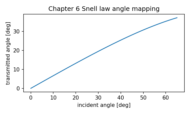
Chapter 7: From One Ray to a Bundle of Rays
One ray is a calculation.
A bundle of rays is an image beginning to form.
In Chapter 6, we finally made a ray bend. It reached a spherical surface, found the local normal, looked up the refractive indices on both sides, and changed direction through vector Snell’s law. That was the first complete refractive event.
But an optical system does not earn much trust from one ray.
One ray can tell us whether the code is alive. It can help debug an intersection. It can show that refraction bends in the right direction. It can expose a sign error. But it cannot tell us how an image forms.
To see image formation, we need many rays.
Not random rays thrown at the lens without thought, but a deliberately sampled bundle:
rays across the pupil
rays from a chosen field point
rays at one or more wavelengths
rays traced to the image plane
When those rays land on the image plane, their transverse coordinates become data. Plot those coordinates, and you get a spot diagram.
That sentence is the core of this chapter:
A spot diagram is not drawn by hand. It is the plotted landing positions of traced rays.
This sounds obvious once stated. But it is worth making explicit, because spot diagrams are often encountered as finished software plots. The learner sees dots. The software hides the ray generation, the pupil sampling, the surface interactions, and the image-plane intercepts.
Here we will not hide them.
We will build the bundle ourselves.
What a spot diagram really contains
A spot diagram is a scatter plot of ray intersections at an image surface.
For each ray that survives the optical system, we record:
x_image
y_image
Then we plot those points.
If the lens were perfect under geometric optics, rays from one object point would land at one image point. The spot would collapse to a point. Real lenses do not do that. Rays from different parts of the pupil land in slightly different places because of aberrations, defocus, field effects, and wavelength effects.
The spot diagram therefore answers a concrete question:
For this field point,
at this wavelength or wavelength set,
through this aperture,
where do sampled rays land on the image plane?
That question has several hidden inputs:
field point
pupil sampling pattern
aperture size
wavelengths
image plane position
lens prescription
material model
ray tracing algorithm
If you do not know those inputs, the plot is hard to interpret.
A tight spot usually suggests good geometric imaging at that field and wavelength. A wide spot suggests blur. A spot stretched in one direction may suggest astigmatism, coma, field effects, or defocus, depending on context. A spot with different colors separated from each other suggests chromatic aberration.
But the plot itself is not the cause. It is the result.
The computation is:
generate rays
→ trace rays through the optical system
→ collect image-plane intercepts
→ plot intercepts
That is what we will build.
From aperture to pupil sampling
To generate a bundle, we need to decide where rays enter the system.
For a simple object-at-infinity example, all rays from one field point enter with the same direction. The rays differ by where they pass through the entrance pupil or, in our simplified early model, where they start on a launch plane before the lens.
Let us start with a normalized pupil coordinate:
(px, py)
where the circular pupil is:
px² + py² <= 1
If the physical pupil radius is R_pupil, then the ray starting coordinates can be:
x = R_pupil px
y = R_pupil py
This gives us a set of ray starting positions across a circular aperture.
There are many ways to sample a pupil:
square grid clipped to a circle
polar grid
rings and spokes
random sampling
quasi-random sampling
Gaussian quadrature
For this chapter, we will use a square grid clipped to a circle. It is not the most elegant sampling method, but it is easy to inspect. That matters more right now.
Here is the function:
import numpy as np
def sample_pupil_grid(samples_per_axis, pupil_radius):
"""Return pupil sample points on a square grid clipped to a circle.
Parameters
----------
samples_per_axis:
Number of grid points along x and y before circular clipping.
pupil_radius:
Physical pupil radius in the same length unit as the lens, usually mm.
Returns
-------
An array of shape (N, 2), containing x, y pupil coordinates.
"""
coords = np.linspace(-pupil_radius, pupil_radius, samples_per_axis)
points = []
for x in coords:
for y in coords:
if x*x + y*y <= pupil_radius*pupil_radius:
points.append((x, y))
return np.array(points, dtype=float)
Test it:
pupil_points = sample_pupil_grid(samples_per_axis=9, pupil_radius=5.0)
print(pupil_points.shape)
print(pupil_points[:5])
This gives a set of points inside a circular aperture of radius 5 mm.
Plot the samples:
import matplotlib.pyplot as plt
plt.scatter(pupil_points[:, 0], pupil_points[:, 1])
plt.gca().set_aspect("equal", adjustable="box")
plt.xlabel("pupil x [mm]")
plt.ylabel("pupil y [mm]")
plt.title("Square-grid pupil sampling clipped to a circle")
plt.show()
This plot is not a spot diagram. It is the input sampling pattern.
That distinction matters.
The pupil plot shows where rays enter the aperture. The spot diagram shows where those rays land after tracing.
Field sampling: where the object point is
A pupil sample tells us where a ray passes through the aperture.
A field point tells us which object point the ray comes from.
For an object at infinity, a field can be represented by an incoming angle. An on-axis field has rays traveling along the optical axis:
θx = 0
θy = 0
An off-axis field may have rays tilted by a few degrees:
θx = 0
θy = 5 degrees
or, depending on coordinate convention, field may be represented in x or y. We will keep a simple two-angle model:
theta_x_deg
theta_y_deg
The direction helper from Chapter 4 was:
import math
def normalize(v):
v = np.asarray(v, dtype=float)
norm = np.linalg.norm(v)
if norm == 0:
raise ValueError("Cannot normalize a zero vector.")
return v / norm
def direction_from_field_angles(theta_x_deg=0.0, theta_y_deg=0.0):
"""Create a ray direction from field angles.
The ray points toward (tan θx, tan θy, 1).
This is a convenient object-at-infinity model.
"""
tx = math.tan(math.radians(theta_x_deg))
ty = math.tan(math.radians(theta_y_deg))
return normalize([tx, ty, 1.0])
For a given field point, all rays in the bundle share this direction. They start from different pupil coordinates, but they are parallel.
That is the object-at-infinity approximation:
same field → same incoming direction
different pupil coordinates → different ray starting positions
This is not the only possible object model. For a finite object, rays would originate from a finite object point and pass through different pupil locations. But object-at-infinity is natural for many optical examples, and it keeps the first spot diagram readable.
Making a ray bundle
Now combine field direction and pupil coordinates.
We choose a launch plane before the first surface:
z_start = -20 mm
For each pupil sample (x, y), create a ray:
position = [x, y, z_start]
direction = direction_from_field_angles(theta_x, theta_y)
wavelength = selected wavelength
Here is the code:
def make_ray_bundle(
pupil_points,
z_start,
theta_x_deg=0.0,
theta_y_deg=0.0,
wavelength_um=0.5875618,
intensity=1.0,
):
"""Create a bundle of rays from pupil samples and field angles."""
direction = direction_from_field_angles(theta_x_deg, theta_y_deg)
rays = []
for x, y in pupil_points:
rays.append(
Ray(
position=[x, y, z_start],
direction=direction,
wavelength_um=wavelength_um,
intensity=intensity,
)
)
return rays
Create an on-axis bundle:
pupil_points = sample_pupil_grid(samples_per_axis=11, pupil_radius=5.0)
rays = make_ray_bundle(
pupil_points=pupil_points,
z_start=-20.0,
theta_x_deg=0.0,
theta_y_deg=0.0,
wavelength_um=0.5875618,
)
print(len(rays))
print(rays[0].position, rays[0].direction)
Now we have many rays.
They do not yet form a spot diagram. They are only the input bundle.
The next step is to trace each one.
Reusing the singlet tracer
From Chapter 6, we had a simple biconvex singlet:
front = IntersectableSurface(
radius=50.0,
z_vertex=0.0,
semi_diameter=10.0,
comment="front surface"
)
back = IntersectableSurface(
radius=-50.0,
z_vertex=5.0,
semi_diameter=10.0,
comment="back surface"
)
image = IntersectableSurface(
radius=float("inf"),
z_vertex=50.0,
semi_diameter=None,
surface_type="plane",
comment="image plane"
)
And a tracing function:
def trace_simple_singlet_ray(ray, front, back, image, glass_material):
n_air = 1.0
n_glass = glass_material.n(ray.wavelength_um)
interact_refractive_surface(ray, front, n1=n_air, n2=n_glass)
if ray.alive:
interact_refractive_surface(ray, back, n1=n_glass, n2=n_air)
if ray.alive:
hit_image = intersect_surface(ray, image)
if hit_image is None:
ray.stop("missed image plane")
else:
ray.propagate(hit_image.t, refractive_index=n_air)
return ray
Now apply it to a bundle:
def trace_bundle_through_singlet(rays, front, back, image, glass_material):
traced = []
for ray in rays:
traced.append(
trace_simple_singlet_ray(
ray,
front=front,
back=back,
image=image,
glass_material=glass_material,
)
)
return traced
Trace:
traced_rays = trace_bundle_through_singlet(
rays,
front=front,
back=back,
image=image,
glass_material=N_BK7,
)
Now every ray has either reached the image plane or stopped somewhere.
Before plotting, we should collect only the rays that survived.
Collecting image-plane intercepts
A spot diagram needs the image-plane positions of valid rays.
def collect_image_points(traced_rays):
"""Return image-plane x, y points from rays that reached the image plane."""
points = []
valid_rays = []
for ray in traced_rays:
if ray.alive:
points.append((ray.position[0], ray.position[1]))
valid_rays.append(ray)
return np.array(points, dtype=float), valid_rays
Use it:
spot_points, valid_rays = collect_image_points(traced_rays)
print("traced rays:", len(traced_rays))
print("valid rays:", len(valid_rays))
print("spot points:", spot_points.shape)
This is the raw data behind a spot diagram.
Do not plot yet. First look at the numbers.
print(spot_points[:10])
You should see x and y positions at the image plane.
For an on-axis rotationally symmetric system, the spot should be centered near the axis if the image plane is close to focus. If the image plane is not at best focus, the spot may form a larger blur circle.
That is not a bug. The image plane location is one of the inputs.
Plotting the first spot diagram
Now we can plot.
def plot_spot(points, title="Spot diagram"):
if len(points) == 0:
raise ValueError("No valid spot points to plot.")
plt.scatter(points[:, 0], points[:, 1], s=12)
plt.axhline(0.0, linewidth=0.5)
plt.axvline(0.0, linewidth=0.5)
plt.gca().set_aspect("equal", adjustable="box")
plt.xlabel("image x [mm]")
plt.ylabel("image y [mm]")
plt.title(title)
plt.show()
plot_spot(spot_points, title="On-axis spot diagram")
There it is.
The plot may be unimpressive at first. It is just dots. Good. We should not rush past that. Those dots are not decorative. They are the final coordinates of rays that were:
generated from pupil samples
propagated to the front surface
refracted into glass
propagated to the back surface
refracted into air
propagated to the image plane
recorded as x, y coordinates
A spot diagram is the visible end of a ray-tracing pipeline.
This is the first real analysis graph we have built from our own computation.
Centered spot diagrams
Many optical software spot diagrams are shown relative to a reference point, such as the chief ray intercept or the centroid of the spot. That makes the shape of the blur easier to inspect.
If the absolute image position is large, the spot may be far from the origin. Centering helps us see the spread.
Two common choices are:
subtract the chief ray intercept
subtract the centroid of all valid ray intercepts
For now, centroid centering is simple:
def center_points_by_centroid(points):
centroid = points.mean(axis=0)
return points - centroid, centroid
Use it:
centered_points, centroid = center_points_by_centroid(spot_points)
print("centroid:", centroid)
plot_spot(centered_points, title="On-axis spot diagram, centered by centroid")
The centered plot tells you the spread pattern. The centroid tells you where the whole bundle landed.
Do not confuse these.
Absolute spot position is useful for image location and distortion.
Centered spot shape is useful for blur and aberration inspection.
Both are data. They answer different questions.
Spot size metrics
A spot diagram is visual, but we often want summary numbers.
A simple one is RMS spot radius.
Given image points (x_i, y_i) and a reference center (x_c, y_c), the RMS radius is:
r_rms = sqrt(mean((x_i - x_c)² + (y_i - y_c)²))
In code:
def rms_spot_radius(points, center=None):
"""Compute RMS spot radius around a center."""
if len(points) == 0:
return np.nan
if center is None:
center = points.mean(axis=0)
shifted = points - center
r2 = shifted[:, 0]**2 + shifted[:, 1]**2
return math.sqrt(float(np.mean(r2)))
Compute it:
rms = rms_spot_radius(spot_points)
print("RMS spot radius [mm]:", rms)
Another simple metric is maximum radius:
def max_spot_radius(points, center=None):
if len(points) == 0:
return np.nan
if center is None:
center = points.mean(axis=0)
shifted = points - center
r = np.sqrt(shifted[:, 0]**2 + shifted[:, 1]**2)
return float(np.max(r))
print("Max spot radius [mm]:", max_spot_radius(spot_points))
These numbers are not replacements for understanding. They are summaries. They tell you how large the traced spot is under the chosen conditions.
Always remember the hidden conditions:
which field
which wavelength
which aperture
which image plane
which pupil sampling
Without those, an RMS spot radius is just a number floating in space.
Chief ray and marginal ray
Now we need two important ray names.
The chief ray is the ray from a field point that passes through the center of the aperture stop.
The marginal ray is often the ray from an on-axis object point that passes through the edge of the aperture stop.
These definitions are simple in words, but they become subtle in real systems because the entrance pupil may not be physically located at the stop surface, especially in multi-element systems. For this chapter’s simplified object-at-infinity model, we can use a practical approximation:
chief ray:
pupil coordinate near (0, 0) for the selected field
marginal ray:
pupil coordinate near the edge of the pupil for the on-axis field
This is enough to learn the computational role.
The chief ray helps define image height for an off-axis field. It is often used as a reference for centering spot diagrams.
The marginal ray helps define aperture behavior and first-order quantities. It tells us how an edge ray behaves.
Let us create them in our simple model.
def make_chief_ray(z_start, theta_x_deg=0.0, theta_y_deg=0.0, wavelength_um=0.5875618):
"""Simplified chief ray: starts at pupil center."""
return Ray(
position=[0.0, 0.0, z_start],
direction=direction_from_field_angles(theta_x_deg, theta_y_deg),
wavelength_um=wavelength_um,
)
def make_marginal_ray(z_start, pupil_radius, wavelength_um=0.5875618):
"""Simplified marginal ray for an on-axis field: starts at pupil edge."""
return Ray(
position=[pupil_radius, 0.0, z_start],
direction=direction_from_field_angles(0.0, 0.0),
wavelength_um=wavelength_um,
)
Trace them:
chief = make_chief_ray(z_start=-20.0, theta_x_deg=0.0, theta_y_deg=3.0)
marginal = make_marginal_ray(z_start=-20.0, pupil_radius=5.0)
trace_simple_singlet_ray(chief, front, back, image, N_BK7)
trace_simple_singlet_ray(marginal, front, back, image, N_BK7)
print("chief image point:", chief.position)
print("marginal image point:", marginal.position)
In a real design program, chief and marginal ray aiming may be more sophisticated. The program may solve for rays that pass through pupil centers and aperture edges after accounting for the optical system before the stop.
But the idea remains:
chief ray → field reference
marginal ray → aperture edge reference
They are special samples inside the larger ray bundle.
Off-axis field spot diagram
Now let us generate a spot for an off-axis field.
For example:
theta_y = 3 degrees
This means all rays enter tilted in the y-z plane. In our simple model, the bundle starts across the pupil and travels with the same tilted direction.
pupil_points = sample_pupil_grid(samples_per_axis=13, pupil_radius=5.0)
off_axis_rays = make_ray_bundle(
pupil_points=pupil_points,
z_start=-20.0,
theta_x_deg=0.0,
theta_y_deg=3.0,
wavelength_um=0.5875618,
)
traced_off_axis = trace_bundle_through_singlet(
off_axis_rays,
front=front,
back=back,
image=image,
glass_material=N_BK7,
)
off_axis_points, valid_off_axis = collect_image_points(traced_off_axis)
plot_spot(off_axis_points, title="Off-axis spot diagram, absolute coordinates")
The spot may be shifted away from the origin because the field is off-axis. That shift is expected. It is the image height.
To inspect blur shape, center it:
off_axis_centered, off_axis_centroid = center_points_by_centroid(off_axis_points)
print("off-axis centroid:", off_axis_centroid)
print("off-axis RMS radius:", rms_spot_radius(off_axis_points))
plot_spot(off_axis_centered, title="Off-axis spot diagram, centered")
The shape may no longer be circular. It may stretch, skew, or form a pattern that hints at off-axis aberrations.
Do not over-diagnose yet. We have not introduced coma, astigmatism, field curvature, or distortion formally. Chapter 9 will do that. For now, it is enough to see that off-axis ray bundles do not necessarily behave like on-axis bundles.
The spot diagram gives us the evidence.
Field series: center to edge
Optical software often shows spot diagrams for several field points. That lets you see how image quality changes from the center to the edge of the field.
We can do a small version.
def spot_for_field(theta_y_deg, samples_per_axis=13, pupil_radius=5.0, wavelength_um=0.5875618):
pupil_points = sample_pupil_grid(samples_per_axis, pupil_radius)
rays = make_ray_bundle(
pupil_points=pupil_points,
z_start=-20.0,
theta_x_deg=0.0,
theta_y_deg=theta_y_deg,
wavelength_um=wavelength_um,
)
traced = trace_bundle_through_singlet(rays, front, back, image, N_BK7)
points, valid = collect_image_points(traced)
return points, valid
for field_angle in [0.0, 1.5, 3.0, 5.0]:
points, valid = spot_for_field(field_angle)
centered, centroid = center_points_by_centroid(points)
print(
f"field {field_angle:.1f} deg: "
f"valid rays={len(valid)}, "
f"centroid={centroid}, "
f"RMS={rms_spot_radius(points):.6f} mm"
)
This is already an optical analysis table.
It tells us, under our simplified setup, how the traced spot changes with field angle.
We can plot each field separately. For the book text, separate plots are often clearer than cramming many fields into one graph. Here is one field at a time:
field_angle = 5.0
points, valid = spot_for_field(field_angle)
centered, centroid = center_points_by_centroid(points)
plot_spot(centered, title=f"Centered spot diagram, field = {field_angle} deg")
This pattern is exactly what commercial software automates. But now we know the data pipeline.
Polychromatic ray bundles
So far, we have traced one wavelength at a time.
A real visible-light spot diagram may include multiple wavelengths. Each wavelength uses its own refractive index through the material model. If the plot colors the rays by wavelength, chromatic separation becomes visible.
Let us create a multi-wavelength bundle.
def make_polychromatic_bundle(
pupil_points,
z_start,
theta_x_deg=0.0,
theta_y_deg=0.0,
wavelengths_um=(0.4861327, 0.5875618, 0.6562725),
):
rays = []
for wl in wavelengths_um:
rays.extend(
make_ray_bundle(
pupil_points=pupil_points,
z_start=z_start,
theta_x_deg=theta_x_deg,
theta_y_deg=theta_y_deg,
wavelength_um=wl,
)
)
return rays
Trace:
wavelengths = [0.4861327, 0.5875618, 0.6562725]
pupil_points = sample_pupil_grid(samples_per_axis=11, pupil_radius=5.0)
poly_rays = make_polychromatic_bundle(
pupil_points=pupil_points,
z_start=-20.0,
theta_x_deg=0.0,
theta_y_deg=0.0,
wavelengths_um=wavelengths,
)
traced_poly = trace_bundle_through_singlet(poly_rays, front, back, image, N_BK7)
Collect points by wavelength:
def collect_points_by_wavelength(traced_rays):
groups = {}
for ray in traced_rays:
if not ray.alive:
continue
wl = ray.wavelength_um
groups.setdefault(wl, []).append((ray.position[0], ray.position[1]))
return {wl: np.array(points, dtype=float) for wl, points in groups.items()}
Plot:
groups = collect_points_by_wavelength(traced_poly)
for wl, points in groups.items():
plt.scatter(points[:, 0], points[:, 1], s=12, label=f"{wl:.4f} µm")
plt.gca().set_aspect("equal", adjustable="box")
plt.xlabel("image x [mm]")
plt.ylabel("image y [mm]")
plt.title("Polychromatic spot diagram")
plt.legend()
plt.show()
This plot may show small wavelength-dependent shifts or spread differences. The exact appearance depends on the lens, aperture, field, and image plane.
The important part is not whether this simple singlet gives a beautiful pattern. It will not. The important part is that chromatic behavior has entered through the computation:
ray.wavelength_um
→ material.n(wavelength)
→ different refraction angles
→ different image-plane intercepts
A polychromatic spot diagram is not magic. It is many monochromatic ray traces plotted together or combined according to a defined rule.
Why the spot changes when the image plane moves
A spot diagram is always tied to an image plane position.
Move the image plane, and the same outgoing rays intersect it at different locations. Near focus, the spot may be small. Before or after focus, the spot may expand.
This is not a display setting. It is geometry.
Let us compute RMS spot radius for different image plane positions.
def rms_for_image_plane(z_image, field_angle=0.0, wavelength_um=0.5875618):
image_surface = IntersectableSurface(
radius=float("inf"),
z_vertex=z_image,
semi_diameter=None,
surface_type="plane",
comment="image plane",
)
pupil_points = sample_pupil_grid(samples_per_axis=13, pupil_radius=5.0)
rays = make_ray_bundle(
pupil_points=pupil_points,
z_start=-20.0,
theta_x_deg=0.0,
theta_y_deg=field_angle,
wavelength_um=wavelength_um,
)
traced = trace_bundle_through_singlet(
rays,
front=front,
back=back,
image=image_surface,
glass_material=N_BK7,
)
points, valid = collect_image_points(traced)
if len(points) == 0:
return np.nan
return rms_spot_radius(points)
Sweep focus:
z_values = np.linspace(35.0, 65.0, 61)
rms_values = [rms_for_image_plane(z) for z in z_values]
plt.plot(z_values, rms_values)
plt.xlabel("image plane z [mm]")
plt.ylabel("RMS spot radius [mm]")
plt.title("RMS spot radius versus image plane position")
plt.show()
This plot is not a spot diagram. It is a focus scan based on spot size.
The minimum suggests a best-focus region according to our chosen RMS criterion.
This is another important software-output lesson:
A spot diagram depends on focus position. A bad-looking spot may mean the lens is bad, or it may mean the image plane is not placed where that analysis expects.
A real optical program may offer several focus definitions. We will study paraxial focus and first-order quantities in Chapter 8, then aberration and best focus more carefully in Chapter 9.
For now, just remember that the image plane is part of the analysis, not an afterthought.
Pupil sampling density changes the plot
A spot diagram with 9 rays and a spot diagram with 169 rays may show the same system, but they will look different.
The underlying optical system has not changed. The sampling has changed.
Let us compare:
for n in [5, 9, 17]:
pupil_points = sample_pupil_grid(samples_per_axis=n, pupil_radius=5.0)
rays = make_ray_bundle(
pupil_points=pupil_points,
z_start=-20.0,
theta_y_deg=3.0,
wavelength_um=0.5875618,
)
traced = trace_bundle_through_singlet(rays, front, back, image, N_BK7)
points, valid = collect_image_points(traced)
centered, centroid = center_points_by_centroid(points)
print(
f"samples_per_axis={n}, "
f"valid rays={len(valid)}, "
f"RMS={rms_spot_radius(points):.6f} mm"
)
plot_spot(centered, title=f"Centered spot, field 3 deg, grid {n}x{n}")
The rough shape should become clearer as sampling density increases. But more samples also cost more computation.
This is a small preview of a major theme in computational optics:
sampling choices affect numerical results and visual interpretation
We will revisit this forcefully in Chapter 14 when we discuss sampling, normalization, and FFT grids. For spot diagrams, the stakes are already visible. A sparse spot can hide structure. A dense spot can reveal it. A poorly chosen pattern can mislead.
The plot is only as honest as the sampling behind it.
A better pupil sampler: rings and angles
A square grid clipped to a circle is easy, but optical ray diagrams often use ring-based sampling. That gives more direct control over radial positions.
Here is a simple polar sampler:
def sample_pupil_polar(num_rings, points_per_ring, pupil_radius, include_center=True):
"""Return pupil points sampled on concentric rings."""
points = []
if include_center:
points.append((0.0, 0.0))
for ring in range(1, num_rings + 1):
r = pupil_radius * ring / num_rings
count = points_per_ring * ring
for j in range(count):
phi = 2.0 * math.pi * j / count
x = r * math.cos(phi)
y = r * math.sin(phi)
points.append((x, y))
return np.array(points, dtype=float)
Plot it:
polar_points = sample_pupil_polar(
num_rings=4,
points_per_ring=6,
pupil_radius=5.0
)
plt.scatter(polar_points[:, 0], polar_points[:, 1])
plt.gca().set_aspect("equal", adjustable="box")
plt.xlabel("pupil x [mm]")
plt.ylabel("pupil y [mm]")
plt.title("Polar pupil sampling")
plt.show()
Now trace it:
rays = make_ray_bundle(
pupil_points=polar_points,
z_start=-20.0,
theta_y_deg=3.0,
wavelength_um=0.5875618,
)
traced = trace_bundle_through_singlet(rays, front, back, image, N_BK7)
points, valid = collect_image_points(traced)
centered, centroid = center_points_by_centroid(points)
plot_spot(centered, title="Centered spot from polar pupil sampling")
The spot may look different from the square-grid version because the pupil samples are different. The lens did not change. The sampling changed.
That is an important lesson. A spot diagram is a sampled view of ray behavior, not the continuous truth itself.
Vignetting and blocked rays
Not every generated ray necessarily reaches the image plane.
A ray may be stopped because:
it misses a surface
it hits outside a clear aperture
it undergoes total internal reflection
it fails to reach the image plane
For a spot diagram, we normally plot only rays that survive to the image plane. But we should also count the lost rays.
def ray_status_counts(rays):
counts = {}
for ray in rays:
key = "alive" if ray.alive else ray.stop_reason
counts[key] = counts.get(key, 0) + 1
return counts
Use it:
counts = ray_status_counts(traced)
print(counts)
If many rays are blocked, the spot diagram alone may not tell the whole story. A tiny spot made from a few surviving rays is not automatically good news. It may mean most of the aperture is being clipped.
This is why optical software often reports vignetting or ray failures separately.
The spot diagram answers:
Where did surviving rays land?
It does not fully answer:
How many rays failed to get there?
You need both.
Reading a spot diagram carefully
A spot diagram can tell you many things, but it can also tempt you to overread.
Here is a careful way to read it.
First, check the conditions:
field point
wavelength or wavelength set
aperture
image plane position
sampling pattern
reference center
units
Second, look at the scale. A spot that looks large on a plot may be tiny in millimeters. A spot that looks small may still be large compared with pixel size or diffraction scale.
Third, ask whether the plot is absolute or centered. Absolute coordinates show image location. Centered coordinates show spread.
Fourth, check whether all rays survived. A clean spot from a heavily clipped bundle can be misleading.
Fifth, compare across fields and wavelengths. A lens may be good on-axis and poor off-axis. It may be good in green and worse in blue or red.
Sixth, remember the limitation:
A geometric spot diagram does not include diffraction.
That last point matters.
A perfect geometric spot can still produce a finite diffraction pattern. Conversely, a small geometric spot does not automatically mean excellent MTF at every spatial frequency. Spot diagrams are useful, but they are not the whole imaging story.
This book is moving toward PSF and MTF precisely because geometric ray landing points are not enough.
But for now, spot diagrams are the right next step. They show what real rays do.
Spot diagram versus ray fan
It is useful to distinguish two common ray-based plots.
A spot diagram plots image-plane landing points:
x_image, y_image
A ray fan plot usually plots transverse ray error versus pupil coordinate:
pupil coordinate → ray error
Both are built from traced rays. They simply organize the results differently.
Spot diagram asks:
Where did the rays land?
Ray fan asks:
How does the landing error vary across the pupil?
Chapter 9 will use ray fans to discuss aberrations more clearly. For now, the spot diagram is the simpler visual result.
But keep the relationship in mind:
same traced rays
different plotted quantities
That is a recurring pattern in optical analysis.
Optiland SpotDiagram comparison
Now let us compare our teaching pipeline with a real library-level call.
In Optiland, the high-level workflow is much shorter. After building or loading an optical system, a spot diagram can be generated through an analysis object.
A compact example looks like this:
from optiland.samples.objectives import CookeTriplet
from optiland.analysis import SpotDiagram
lens = CookeTriplet()
spot = SpotDiagram(lens)
spot.view()
For a custom singlet, the workflow follows the same spirit:
from optiland import optic
from optiland.analysis import SpotDiagram
lens = optic.Optic()
lens.surfaces.add(index=0, radius=float("inf"), thickness=float("inf"))
lens.surfaces.add(index=1, radius=50.0, thickness=5.0, material="N-BK7", is_stop=True)
lens.surfaces.add(index=2, radius=-50.0, thickness=45.0)
lens.surfaces.add(index=3)
lens.set_aperture(aperture_type="EPD", value=10.0)
lens.fields.set_type("angle")
lens.fields.add(y=0.0)
lens.fields.add(y=3.0)
lens.wavelengths.add(value=0.5876, is_primary=True)
spot = SpotDiagram(lens)
spot.view()
Exact options and method signatures may vary by version, so treat this as the conceptual comparison rather than a promise about every installed environment.
The important point is what the library call hides.
When you call:
spot = SpotDiagram(lens)
spot.view()
the library must do some version of this:
read fields
read wavelengths
read aperture definition
generate ray samples
trace rays through all surfaces
collect image-plane intercepts
plot the points
That is the same pipeline we built manually.
The difference is that Optiland provides the full framework, better surface handling, proper system bookkeeping, and analysis tools. Our code is a teaching skeleton. It exists to make the calculation visible.
We are not replacing the library. We are identifying the calculations the library performs when the plot appears.
Why our plot may not match Optiland exactly
If you compare our spot diagram with Optiland’s and they differ, do not panic.
There are many possible reasons:
different pupil sampling
different ray aiming
different aperture definition
different image plane handling
different material data
different wavelength convention
different field coordinate convention
different focus solve
different normalization or centering
This is not a failure of the comparison. It is part of the lesson.
Optical analysis is full of conventions. A spot diagram is not just “the spot diagram.” It is a spot diagram under specified conditions.
To make a fair comparison, you must match:
lens prescription
surface signs
glass model
wavelengths
aperture type and value
field type and value
image surface position
ray sampling pattern
plot centering convention
That is a lot. It is also exactly why understanding the computation matters.
If all you have is the final plot, you may not know which convention caused the difference.
If you understand the pipeline, you know where to look.
A compact bundle trace summary
Let us gather the chapter’s essential code path in one place.
# 1. Choose pupil sampling.
pupil_points = sample_pupil_grid(samples_per_axis=13, pupil_radius=5.0)
# 2. Choose field and wavelength.
theta_y_deg = 3.0
wavelength_um = 0.5875618
# 3. Generate rays.
rays = make_ray_bundle(
pupil_points=pupil_points,
z_start=-20.0,
theta_x_deg=0.0,
theta_y_deg=theta_y_deg,
wavelength_um=wavelength_um,
)
# 4. Trace rays.
traced_rays = trace_bundle_through_singlet(
rays,
front=front,
back=back,
image=image,
glass_material=N_BK7,
)
# 5. Collect image-plane intercepts.
spot_points, valid_rays = collect_image_points(traced_rays)
# 6. Center and summarize.
centered_points, centroid = center_points_by_centroid(spot_points)
rms_radius = rms_spot_radius(spot_points)
print("valid rays:", len(valid_rays))
print("centroid:", centroid)
print("RMS spot radius:", rms_radius)
# 7. Plot.
plot_spot(centered_points, title="Centered spot diagram")
This is the entire spot diagram pipeline in miniature.
It is short because the earlier chapters have already done their work.
That is the pleasure of building the chain carefully. Once the pieces are in place, the analysis function is not mysterious.
What this chapter adds to the full computation chain
At the beginning of the book, the chain was:
lens prescription
→ surfaces and materials
→ real ray tracing
→ paraxial reference
→ pupil sampling
→ optical path difference
→ pupil function
→ point spread function
→ optical transfer function
→ modulation transfer function
This chapter fills in a crucial part of “real ray tracing” and introduces pupil sampling as a deliberate computational action.
We can now say:
lens prescription defines surfaces
material model defines n(λ)
ray object carries position, direction, and wavelength
intersection finds hit points
vector Snell computes new directions
pupil sampling generates many rays
field sampling sets incoming direction
image-plane intercepts produce spot diagrams
That is a real computational path from data to plot.
No MTF yet. No PSF yet. No wavefront yet. But the foundation is no longer abstract.
You can generate rays, trace them, and plot where they land.
That is one of the first moments when optical software begins to feel less like an oracle and more like a collection of understandable algorithms.
Common mistakes when generating ray bundles
Let us collect the traps.
Mistake 1: Confusing pupil plot with spot plot
The pupil plot shows where rays start or pass through the aperture.
The spot plot shows where traced rays land on the image plane.
They are not the same plot.
Mistake 2: Forgetting the field direction
For an object at infinity, different field points mean different incoming directions. If every bundle uses the same direction, you are only testing one field.
Mistake 3: Comparing spot diagrams with different sampling
A 5-by-5 pupil grid and a 21-by-21 pupil grid may show different visual structure. Match sampling before comparing plots.
Mistake 4: Ignoring blocked rays
A spot diagram of surviving rays should be read together with ray failure counts. A small spot after severe clipping can be misleading.
Mistake 5: Forgetting image plane position
Move the image plane, and the spot changes. A large spot may indicate defocus, not only aberration.
Mistake 6: Mixing absolute and centered coordinates
Absolute spot plots show image position. Centered plots show spread. Know which one you are looking at.
Mistake 7: Treating spot diagrams as diffraction results
Spot diagrams are geometric ray results. They do not show diffraction blur. They are important, but they are not PSF or MTF.
Mistake 8: Calling the chief ray “the center ray” without field context
For a simple on-axis setup, the chief ray may look like the central ray. For off-axis fields and real pupil definitions, chief ray meaning is tied to the aperture stop and field point.
Mistake 9: Over-interpreting a simple teaching lens
Our singlet is a learning system. It is not optimized. If the spots look ugly, that may be the correct result.
The purpose here is to understand the computation, not to pretend a simple biconvex lens is a modern imaging objective.
What you should be able to do now
You should now be able to explain a spot diagram without saying:
The software draws it.
A better answer is:
The program samples rays across the pupil for a selected field and wavelength, traces those rays through the lens using ray-surface intersections and Snell refraction, records where the surviving rays hit the image plane, and plots those intercepts.
That sentence contains the whole chapter.
You should also be able to identify the main inputs:
pupil sampling
field angle
wavelength
aperture
image plane
lens prescription
material model
And you should be able to write a minimal Python version that produces the plot.
That is a meaningful milestone.
The road ahead
We have now completed the first working version of real ray tracing.
But real ray tracing alone is not enough to understand an optical system.
In the next chapter, we will deliberately step backward into approximation.
That may sound strange. After working so hard to trace real rays, why go back to paraxial optics?
Because paraxial optics gives us the skeleton of the system.
Real rays show what actually happens. Paraxial rays show the first-order structure: focal length, image position, F-number, magnification, and principal behavior near the axis.
Without that skeleton, spot diagrams can become isolated pictures. You may see that rays spread, but not know what they are spreading around. You may see that focus changes, but not know the first-order focus reference. You may trace many rays, but not know the system’s basic optical power.
So Chapter 8 will introduce paraxial optics not as an old-fashioned detour, but as the coordinate system of understanding.
The real-ray tracer tells us where rays actually go.
Paraxial optics tells us what the system was trying to do in the first place.
Generated validation figure
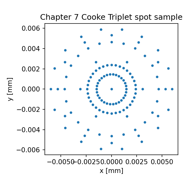
Chapter 8: Why Paraxial Optics Still Matters
We have just built real ray tracing.
That feels like progress, and it is. A ray can now start from a pupil coordinate, travel to a spherical surface, find the local normal, refract through glass, leave the lens, and land on an image plane. A bundle of such rays can produce a spot diagram.
So it may feel odd to step backward now.
Why talk about paraxial optics after real rays?
Why return to thin lenses, small angles, focal length, F-number, numerical aperture, and ABCD matrices when we already have a more exact ray tracer?
Because paraxial optics is not a primitive substitute for real ray tracing.
It is the skeleton.
Real ray tracing tells us what the rays actually do. Paraxial optics tells us what the system is trying to do in first-order form. Without that skeleton, spot diagrams can become isolated pictures. You may see that rays spread, but not know what they are spreading around. You may see that focus changes, but not know which first-order focus the real rays are departing from.
A spot diagram says:
Here is where sampled real rays landed.
Paraxial optics says:
Here is the ideal first-order image structure the system is organized around.
Both are needed.
This chapter introduces the paraxial reference system: ray height, ray slope, transfer matrices, thin lenses, effective focal length, back focal length, F-number, numerical aperture, and magnification. The model stays deliberately small. It gives us the reference frame needed for the next chapter, not a replacement for an optical design textbook.
Chapter 9 will ask:
Why do real rays depart from paraxial rays?
That question is the beginning of aberration.
So first we need to understand the paraxial ray.
A paraxial ray is a reduced description
A real ray in our code carries a 3D position and a 3D direction:
position = [x, y, z]
direction = [dx, dy, dz]
A paraxial ray is simpler.
In one transverse plane, it can be represented by:
y = ray height
u = ray angle or slope
Here y is the height above the optical axis, and u is the small angle the ray makes with the optical axis.
For small angles:
sin u ≈ u
tan u ≈ u
when u is measured in radians.
That small-angle approximation is the heart of paraxial optics.
This approximation does not mean paraxial optics is careless. It means paraxial optics intentionally studies rays close to the optical axis and close to small angles. That is enough to reveal the first-order behavior of the system.
A real ray answers:
Where does this actual ray go through the actual surface?
A paraxial ray answers:
How does a near-axis ray behave under the first-order approximation?
Those are different questions.
Both are useful.
The paraxial ray vector
We will write a paraxial ray as a two-element vector:
[y, u]
where:
y = height above the optical axis, in mm
u = slope or small angle, in radians
In code:
from dataclasses import dataclass
import numpy as np
import math
@dataclass
class ParaxialRay:
y: float
u: float # radians, or slope under small-angle approximation
def as_vector(self):
return np.array([self.y, self.u], dtype=float)
@classmethod
def from_vector(cls, v):
return cls(y=float(v[0]), u=float(v[1]))
A ray traveling parallel to the optical axis at height 5 mm is:
ray = ParaxialRay(y=5.0, u=0.0)
A ray crossing the axis with a small downward angle might be:
ray = ParaxialRay(y=5.0, u=-0.05)
This is much less information than a real ray. That is the point. The paraxial ray is a simplified carrier of first-order behavior.
Propagation in paraxial form
If a paraxial ray travels a distance d through a uniform medium, its height changes according to its slope:
y_new = y + d u
Its slope remains the same:
u_new = u
That can be written as a matrix:
[ y_new ] [ 1 d ] [ y ]
[ u_new ] = [ 0 1 ] [ u ]
This is the first ABCD matrix.
The propagation matrix is:
T(d) = [[1, d],
[0, 1]]
In code:
def translation_matrix(distance):
"""Paraxial propagation through distance d in a uniform medium."""
return np.array([
[1.0, distance],
[0.0, 1.0],
], dtype=float)
def apply_matrix(M, ray):
"""Apply a 2x2 paraxial matrix to a ParaxialRay."""
return ParaxialRay.from_vector(M @ ray.as_vector())
Test it:
ray = ParaxialRay(y=5.0, u=-0.1)
M = translation_matrix(20.0)
out = apply_matrix(M, ray)
print(out)
The result should be:
y = 3.0
u = -0.1
because:
5 + 20 × (-0.1) = 3
This is not a rough drawing. It is the first-order ray transfer written as code.
A thin lens matrix
A thin lens changes the slope of a ray but not its height at the lens plane.
For a thin lens with focal length f in air:
y_new = y
u_new = u - y / f
The matrix is:
L(f) = [[1, 0],
[-1/f, 1]]
In code:
def thin_lens_matrix(focal_length):
"""Thin lens matrix in air."""
f = float(focal_length)
if f == 0:
raise ValueError("Focal length cannot be zero.")
return np.array([
[1.0, 0.0],
[-1.0 / f, 1.0],
], dtype=float)
Test a parallel ray hitting a 50 mm thin lens at height 5 mm:
ray = ParaxialRay(y=5.0, u=0.0)
L = thin_lens_matrix(50.0)
out = apply_matrix(L, ray)
print(out)
The outgoing slope is:
u_new = -5 / 50 = -0.1
That means the ray now travels downward toward the axis. If it propagates 50 mm, it reaches the axis:
T = translation_matrix(50.0)
after_focus = apply_matrix(T, out)
print(after_focus)
The height should be near zero.
This is the paraxial version of focusing.
It is not using real surface intersections. It is not using the exact spherical surface normals. It is using the first-order model of a lens.
That is why it is so compact.
Matrix multiplication is the optical system
An optical system can be represented as a product of paraxial matrices.
If a ray passes through:
translation d1
thin lens f
translation d2
then:
ray_out = T(d2) L(f) T(d1) ray_in
The rightmost matrix acts first.
So the system matrix is:
M = T(d2) @ L(f) @ T(d1)
In code:
def system_matrix(*matrices):
"""Combine matrices in the order they act on the ray.
system_matrix(A, B, C) returns C @ B @ A if the ray sees A first,
then B, then C.
"""
M = np.eye(2)
for element in matrices:
M = element @ M
return M
This version lets us write elements in physical order:
M = system_matrix(
translation_matrix(10.0),
thin_lens_matrix(50.0),
translation_matrix(40.0),
)
The ray sees 10 mm of propagation, then the lens, then 40 mm more propagation.
This order convention is worth being explicit about. Matrix optics is compact, but order matters. Swapping two elements changes the system.
The ABCD matrix
A general first-order system matrix is written:
M = [[A, B],
[C, D]]
It maps input ray height and slope to output ray height and slope:
[ y_out ] [ A B ] [ y_in ]
[ u_out ] = [ C D ] [ u_in ]
So:
y_out = A y_in + B u_in
u_out = C y_in + D u_in
Each coefficient has a meaning.
A tells how input height contributes to output height.
B tells how input angle contributes to output height.
C tells how input height contributes to output angle.
D tells how input angle contributes to output angle.
The most important coefficient for optical power is often C.
For a thin lens:
M = [[1, 0],
[-1/f, 1]]
so:
C = -1/f
That is why, for a system in air, the effective focal length is often obtained from:
EFL = -1 / C
when C is not zero.
Let us write that.
def matrix_elements(M):
A, B = M[0, 0], M[0, 1]
C, D = M[1, 0], M[1, 1]
return A, B, C, D
def effective_focal_length(M):
"""Effective focal length for a system in air using [y, u] convention."""
A, B, C, D = matrix_elements(M)
if abs(C) < 1e-12:
return math.inf
return -1.0 / C
Test it:
L = thin_lens_matrix(50.0)
print(effective_focal_length(L))
It should print 50.0.
That is reassuring. A 50 mm thin lens has 50 mm effective focal length in this simplified model.
Back focal length
Effective focal length and back focal length are related but not always identical.
Effective focal length is tied to the system’s optical power and principal planes. Back focal length is the distance from the last surface or last reference plane to the rear focal point.
For a system matrix M = [[A, B], [C, D]], consider an incoming collimated ray:
u_in = 0
After the system:
y_out = A y_in
u_out = C y_in
Now let the ray propagate a distance s after the system. Its height becomes:
y(s) = y_out + s u_out
The rear focal point is where this collimated input ray crosses the axis:
0 = A y_in + s C y_in
For nonzero y_in:
s = -A / C
So, in this simple same-medium convention:
BFL = -A / C
Write it:
def back_focal_length(M):
"""Back focal length from the output reference plane, in air."""
A, B, C, D = matrix_elements(M)
if abs(C) < 1e-12:
return math.inf
return -A / C
For a thin lens whose reference plane is at the lens itself:
L = thin_lens_matrix(50.0)
print("EFL:", effective_focal_length(L))
print("BFL:", back_focal_length(L))
Both are 50 mm.
Now add a translation after the lens into the system matrix:
M = system_matrix(
thin_lens_matrix(50.0),
translation_matrix(10.0),
)
print(M)
print("EFL:", effective_focal_length(M))
print("BFL from output plane:", back_focal_length(M))
The effective focal length remains 50 mm, because the optical power did not change. But the back focal length measured from the new output plane changes. If the output plane is 10 mm after the thin lens, the remaining distance to focus is about 40 mm.
This is a crucial distinction.
A system can have the same effective focal length but a different back focal length depending on where the last reference plane or last surface is.
That is why optical prescriptions care about surface positions, not just power.
Thin lens formula from matrices
The familiar thin lens formula is:
1/s + 1/s' = 1/f
where:
s = object distance before the lens
s' = image distance after the lens
f = focal length
Sign conventions vary, so this formula is often a source of confusion. Instead of arguing with signs abstractly, let us derive a simple case using matrices.
Suppose an object point is a distance s before a thin lens. A ray leaves the object point at height 0 and reaches the lens at height y. Its slope at the lens is approximately:
u = y / s
After the thin lens:
u_after = u - y/f
= y/s - y/f
For the ray to reach the image point on the axis after distance s':
0 = y + s' u_after
Substitute:
0 = y + s'(y/s - y/f)
Divide by y:
0 = 1 + s'(1/s - 1/f)
Rearrange:
1/s' = 1/f - 1/s
or:
1/s + 1/s' = 1/f
under this positive-distance setup.
In code:
def thin_lens_image_distance(object_distance, focal_length):
"""Return image distance s' for a thin lens with object distance s.
Uses 1/s + 1/s' = 1/f.
Assumes a simple real-object, real-image positive distance convention.
"""
s = float(object_distance)
f = float(focal_length)
denom = 1.0 / f - 1.0 / s
if abs(denom) < 1e-12:
return math.inf
return 1.0 / denom
Test:
for s in [100.0, 200.0, 1000.0, math.inf]:
if math.isinf(s):
sp = 50.0
else:
sp = thin_lens_image_distance(s, 50.0)
print("object distance:", s, "image distance:", sp)
As the object moves farther away, the image distance approaches the focal length.
This is one of the reasons object-at-infinity examples are so convenient. Parallel incoming rays focus at the focal plane in the paraxial thin-lens model.
Magnification
For a thin lens with object distance s and image distance s', transverse magnification is:
m = -s' / s
The minus sign indicates image inversion under the usual real-object, real-image convention.
In code:
def thin_lens_magnification(object_distance, image_distance):
return -image_distance / object_distance
Example:
s = 100.0
f = 50.0
sp = thin_lens_image_distance(s, f)
m = thin_lens_magnification(s, sp)
print("s' =", sp)
print("m =", m)
For s = 100 mm and f = 50 mm, the image distance is 100 mm and magnification is -1.
Again, this is a first-order result. Real lenses may have distortion, field curvature, aberrations, and finite thickness effects. But the paraxial magnification gives the reference structure.
Without it, “distortion” has no clear meaning. Distortion is not merely “the image looks weird.” It is a departure from the expected paraxial mapping between object field and image position.
We will return to this in Chapter 9.
F-number
F-number is one of the most common optical quantities.
For a lens focused at infinity, a useful first-order definition is:
F/# = f / D
where:
f = effective focal length
D = entrance pupil diameter
A 50 mm lens with a 10 mm entrance pupil diameter has:
F/# = 50 / 10 = 5
or f/5.
In code:
def f_number(effective_focal_length, entrance_pupil_diameter):
D = float(entrance_pupil_diameter)
if D <= 0:
raise ValueError("Entrance pupil diameter must be positive.")
return effective_focal_length / D
Use it:
f = 50.0
D = 10.0
print(f_number(f, D))
This is simple, but it connects directly to ray bundles.
The entrance pupil diameter controls the cone of rays. A larger aperture means a faster system, smaller F-number, and generally stronger demands on aberration correction. A smaller aperture means a slower system, larger F-number, and often reduced geometric aberrations, but more diffraction blur.
This is one of the places where geometric and diffraction thinking meet.
A large aperture may improve light collection and diffraction-limited resolution, but it also asks the lens to handle more extreme rays. If the design is not corrected, real-ray aberrations may dominate.
F-number is therefore not just a label on a camera lens. It is a first-order summary of aperture relative to focal length.
Numerical aperture
Numerical aperture, or NA, describes the cone angle of light.
In image space, for a medium of refractive index n:
NA = n sin θ
where θ is the marginal ray angle relative to the optical axis.
For small angles in air:
NA ≈ sin θ ≈ θ
There is also a common approximate relationship for systems in air:
NA ≈ 1 / (2 F/#)
when the system is focused at infinity and the angles are not too large.
Let us implement both.
def numerical_aperture(n_medium, marginal_angle_rad):
return n_medium * math.sin(marginal_angle_rad)
def na_from_f_number(fno):
return 1.0 / (2.0 * fno)
For a 50 mm focal length and 10 mm entrance pupil diameter:
fno = f_number(50.0, 10.0)
print("F/#:", fno)
print("approx NA:", na_from_f_number(fno))
The approximate NA is 0.1.
This corresponds to a marginal ray angle of about 0.1 radian in the paraxial approximation.
Again, this is first-order. At high NA, exact definitions and sine behavior matter more. But for many introductory optical systems, this approximation gives a useful scale.
F-number connects to the marginal ray
Let us connect F-number to a paraxial ray.
For an object at infinity, a marginal ray enters parallel to the optical axis at pupil height:
y = D / 2
After a thin lens of focal length f, its slope becomes:
u = -y / f = -(D/2) / f
So the marginal ray angle magnitude is approximately:
|u| = D / (2f) = 1 / (2 F/#)
That is the same approximate NA in air.
This is a nice moment because it links several quantities:
pupil diameter
focal length
F-number
marginal ray slope
numerical aperture
They are not separate facts to memorize. They are different views of the first-order cone of light.
In code:
def marginal_slope_from_f_and_d(f, D):
return -(D / 2.0) / f
f = 50.0
D = 10.0
u_marginal = marginal_slope_from_f_and_d(f, D)
print("marginal slope:", u_marginal)
print("approx NA:", abs(u_marginal))
print("from F/#:", na_from_f_number(f_number(f, D)))
The numbers agree under the paraxial approximation.
This is exactly why paraxial optics is useful. It compresses the geometry into relationships you can reason with.
Real ray marginal behavior versus paraxial marginal behavior
Now connect this chapter to the previous one.
In the real ray tracer, a marginal ray at the edge of the pupil hits the spherical surface at a different normal than a near-axis ray. It refracts according to exact geometry.
In paraxial optics, the marginal ray is represented by a height and a small slope. The lens changes its slope linearly:
u_new = u - y/f
If the ray is near the axis and the angle is small, the two descriptions should be close.
If the ray is far from the axis or the lens has significant aberration, the real ray departs from the paraxial prediction.
That departure is not an inconvenience. It is the beginning of aberration analysis.
A real ray trace gives:
actual image-plane intercept
A paraxial model gives:
first-order expected intercept
The difference gives:
transverse ray error
Chapter 9 will build directly on that idea.
A paraxial focus scan
Let us make a small paraxial focus calculation using matrices.
A collimated ray entering a thin lens at height y should cross the axis at the focal distance. We can verify this by propagating to different z positions and measuring height.
def trace_paraxial_thin_lens_to_plane(y_in, u_in, f, z_after_lens):
ray = ParaxialRay(y=y_in, u=u_in)
ray_after_lens = apply_matrix(thin_lens_matrix(f), ray)
ray_at_plane = apply_matrix(translation_matrix(z_after_lens), ray_after_lens)
return ray_at_plane
Sweep image plane position:
f = 50.0
y_in = 5.0
u_in = 0.0
z_values = np.linspace(30.0, 70.0, 9)
for z in z_values:
out = trace_paraxial_thin_lens_to_plane(y_in, u_in, f, z)
print(f"z={z:.1f} mm, y={out.y:.4f} mm")
At z = 50 mm, the height should be close to zero.
This is the paraxial version of a focus scan. It uses one marginal ray rather than a full bundle. For a thin lens, the result is exact within the paraxial model.
In a real spherical singlet, the edge ray may not cross at exactly the same point as the near-axis ray. That difference is spherical aberration.
Again, paraxial optics gives the reference.
A simple thick-lens approximation with matrices
A real singlet has two surfaces and thickness. We can build a first-order model from refractions and translations too, but the cleanest matrix form depends on the choice of ray variables.
There are two common conventions:
[y, u]
[y, n u]
The second is often called the reduced-angle convention. It makes refraction matrices especially clean across media with different refractive index.
To keep this chapter readable, we will not build a full thick-lens refraction matrix system with changing media. That deserves careful sign conventions and would distract from the main purpose.
Instead, we will do two things:
- use thin-lens matrices for clear first-order intuition;
- use the matrix results as a reference concept for real ray tracing.
This is an intentional boundary.
This chapter does not replace an optical design program’s paraxial engine. It shows what that engine is trying to compute.
A production optical library can calculate first-order properties from the full sequential system, including surface powers, thickness, refractive indices, stops, pupils, and principal planes. Our teaching code shows the skeleton.
That skeleton is enough to understand the outputs.
Principal planes, without pretending they are simple drawings
For a thin lens, the principal planes sit at the lens plane. That is why focal length and back focal length are the same.
For a thick lens or multi-element system, the effective optical power behaves as if it were associated with principal planes that may lie inside or outside the physical glass.
This is why:
EFL and BFL can differ
Effective focal length is measured from a principal plane. Back focal length is measured from the last surface or output reference plane.
This distinction matters in practical design.
A lens may have a long effective focal length but a short back focal length. Or it may be designed to have a long back focal distance to leave room for a mirror, sensor package, filter, shutter, or mechanical mount.
If you only know the focal length, you do not know where the image plane sits relative to the final glass surface.
The paraxial system matrix helps compute these first-order distances.
In our same-medium ABCD model:
EFL = -1 / C
BFL = -A / C
The difference between those two values indicates that the rear principal plane is not at the output reference plane.
This is not just terminology. It affects layout.
An example where EFL and BFL differ
Let us make a simple system: a thin lens, then a 10 mm translation to the output reference plane.
M = system_matrix(
thin_lens_matrix(50.0),
translation_matrix(10.0),
)
A, B, C, D = matrix_elements(M)
print("M =")
print(M)
print("A, B, C, D =", A, B, C, D)
print("EFL:", effective_focal_length(M))
print("BFL:", back_focal_length(M))
The effective focal length is still 50 mm. The back focal length from the output plane is 40 mm.
Nothing about the lens power changed. Only the reference plane moved 10 mm downstream.
This example is simple, but it teaches a real lesson:
First-order quantities are always tied to reference planes.
When optical software reports EFL, BFL, FFL, principal plane positions, or pupil locations, it is doing paraxial bookkeeping. Those values are not decorative labels. They tell you how the system is organized.
Field angle and image height
For an object at infinity, a paraxial image height is approximately:
y_image ≈ f tan θ
For small angles:
tan θ ≈ θ
so:
y_image ≈ f θ
where θ is in radians.
In code:
def paraxial_image_height_from_field(focal_length, field_angle_deg):
theta = math.radians(field_angle_deg)
return focal_length * math.tan(theta)
Example:
for angle in [0.0, 1.0, 3.0, 5.0]:
print(angle, paraxial_image_height_from_field(50.0, angle))
This is the first-order image height.
Now connect this to Chapter 7. For an off-axis spot diagram, the centroid or chief-ray intercept may appear at some image height. The paraxial image height gives a reference for where we expect that field point to land.
If the real chief ray lands somewhere different from the paraxial prediction, that difference is related to distortion.
We are not ready to analyze distortion fully yet. But the relationship is already visible:
field angle
→ paraxial image height
→ real chief ray image height
→ distortion comparison
This is another reason paraxial optics matters. It gives meaning to “departure.”
A first-order layout is not an image-quality result
This is important enough to say plainly.
A paraxial design can look good and still make a poor image.
First-order optics can tell you:
rough focal length
image distance
magnification
F-number
NA
pupil relationships
field height
It cannot by itself tell you:
spherical aberration
coma
astigmatism
field curvature
distortion details
chromatic blur
PSF
MTF
Those require real ray tracing and wavefront or diffraction analysis.
So paraxial optics is not the final judge of image quality.
But it is still the skeleton. If the first-order system is wrong, later analysis may be solving the wrong problem.
A lens with the wrong focal length is not rescued by a beautiful MTF plot at a different scale. A design with insufficient back focal distance may be optically interesting but mechanically unusable. A system with the wrong F-number may not meet light-gathering or diffraction requirements.
First-order design sets the stage.
Real-ray and wave-optics analysis tell us how well the system performs on that stage.
A small paraxial design function
Let us write a compact function that summarizes a thin-lens design from focal length and pupil diameter.
@dataclass
class ThinLensFirstOrder:
focal_length: float
entrance_pupil_diameter: float
@property
def efl(self):
return self.focal_length
@property
def fno(self):
return f_number(self.efl, self.entrance_pupil_diameter)
@property
def approx_na(self):
return na_from_f_number(self.fno)
def image_height(self, field_angle_deg):
return paraxial_image_height_from_field(self.efl, field_angle_deg)
def marginal_ray_slope(self):
return marginal_slope_from_f_and_d(self.efl, self.entrance_pupil_diameter)
Use it:
design = ThinLensFirstOrder(
focal_length=50.0,
entrance_pupil_diameter=10.0,
)
print("EFL:", design.efl)
print("F/#:", design.fno)
print("Approx NA:", design.approx_na)
print("Marginal slope:", design.marginal_ray_slope())
for field in [0.0, 3.0, 5.0]:
print("field", field, "image height", design.image_height(field))
This is not a lens optimization tool. It is a first-order calculator.
But even this small class gives useful expectations:
How fast is the system?
How large is the image height?
What marginal cone angle should we expect?
Where should parallel rays focus?
These expectations help us read real-ray outputs.
Comparing paraxial and real focus
Let us connect directly to the singlet from Chapters 6 and 7.
Our real singlet had:
front radius = +50 mm
back radius = -50 mm
center thickness = 5 mm
material = N-BK7
A crude thin-lens estimate for a biconvex lens in air is:
1/f ≈ (n - 1)(1/R1 - 1/R2)
For R1 = +50, R2 = -50, and n ≈ 1.5168:
def thin_lens_focal_length_from_radii(n, R1, R2):
power = (n - 1.0) * (1.0 / R1 - 1.0 / R2)
if abs(power) < 1e-12:
return math.inf
return 1.0 / power
n_bk7_d = N_BK7.n(0.5875618)
f_est = thin_lens_focal_length_from_radii(n_bk7_d, R1=50.0, R2=-50.0)
print("thin-lens estimated focal length:", f_est)
This estimate will be near 48 mm. It ignores thickness, exact principal planes, and real spherical ray behavior, but it gives a scale.
In Chapter 7, if you swept the image plane position and found an RMS spot minimum somewhere near that scale, that should feel reasonable. If the best focus were at 500 mm or 5 mm, you would suspect a sign, unit, or tracing error.
That is another practical use of paraxial optics:
It gives you sanity checks.
A paraxial estimate does not have to be perfect to be useful. It tells you whether the real-ray result is in the right neighborhood.
Matrix code for a thin lens focus check
Now use the estimated focal length as a thin lens and compare paraxial image height across field.
f_est = thin_lens_focal_length_from_radii(n_bk7_d, R1=50.0, R2=-50.0)
D = 10.0
design = ThinLensFirstOrder(
focal_length=f_est,
entrance_pupil_diameter=D,
)
print("Estimated EFL:", design.efl)
print("Estimated F/#:", design.fno)
print("Estimated NA:", design.approx_na)
for field in [0.0, 1.0, 3.0, 5.0]:
print(
f"field={field:.1f} deg, "
f"paraxial image height={design.image_height(field):.4f} mm"
)
Now you have first-order expectations for the same kind of field angles used in the spot diagrams.
This helps you avoid a common beginner confusion.
When an off-axis spot appears away from the origin, that is not automatically an aberration. Much of that displacement is simply image height. Aberration is the departure from the ideal image point, not the existence of image height itself.
That is why centered spot diagrams are useful for blur shape, while absolute spot diagrams are useful for image location.
Paraxial optics tells you what “ideal image location” means.
Optiland paraxial analysis as the higher-level version
A real optical design library does not need our hand-written thin-lens shortcuts. It can compute paraxial properties from the actual sequential model.
For an Optiland system, the high-level idea is:
from optiland import optic
lens = optic.Optic()
lens.surfaces.add(index=0, radius=float("inf"), thickness=float("inf"))
lens.surfaces.add(index=1, radius=50.0, thickness=5.0, material="N-BK7", is_stop=True)
lens.surfaces.add(index=2, radius=-50.0, thickness=45.0)
lens.surfaces.add(index=3)
lens.set_aperture(aperture_type="EPD", value=10.0)
lens.fields.set_type("angle")
lens.fields.add(y=0.0)
lens.wavelengths.add(value=0.5876, is_primary=True)
# Schematic example:
# Inspect paraxial or first-order properties using the library's analysis tools.
# Exact property names may vary by Optiland version.
Depending on the installed version, paraxial properties may be exposed through analysis classes, system properties, or dedicated methods. The exact API is less important than the conceptual comparison.
The library-level paraxial engine should be able to answer questions like:
What is the effective focal length?
What is the back focal length?
What is the F-number?
Where are the principal planes?
What is the paraxial image height?
What is the aperture relationship?
Our teaching code answers a smaller version of those questions for thin lenses and simple ABCD systems.
That is exactly the two-rail method of this book:
minimal code → understand the skeleton
Optiland workflow → see the practical tool
Do not confuse them. Our code is not trying to become a complete paraxial analysis package. It is trying to make the outputs legible.
Why paraxial results may not match simple thin-lens estimates
If you compare a library’s paraxial result for a real singlet with our thin-lens estimate, the numbers may differ.
That is expected.
Reasons include:
finite lens thickness
principal plane shifts
exact refractive index used by the glass catalog
wavelength selection
surface sign convention
reference plane definitions
aperture definition
medium before and after the system
A thin-lens equation is an approximation. A full paraxial analysis of a thick sequential system is still first-order, but it includes more of the actual prescription.
So the hierarchy is:
thin-lens estimate:
quick scale and sanity check
ABCD matrix model:
first-order system behavior under chosen elements
library paraxial analysis:
first-order properties from the actual prescription
real ray tracing:
exact geometric behavior of sampled rays
wavefront / PSF / MTF:
diffraction-aware imaging analysis
Each layer has a job.
Problems appear when we ask one layer to do another layer’s job.
Paraxial optics as a debugging tool
Paraxial optics is not only theory. It is also a debugging tool.
If your real ray tracer gives strange results, paraxial estimates can help isolate the problem.
For example:
Case 1: Focus is wildly wrong
If a simple biconvex lens should have focal length near 50 mm, but your real rays focus near 5000 mm, check:
radius units
refractive index
surface sign
normal direction
Snell n1/n2 order
image plane units
Case 2: Off-axis image height is wrong by a large factor
Check:
field angle units
degrees versus radians
direction vector construction
image plane position
coordinate convention
Case 3: F-number does not match ray cone
Check:
aperture diameter versus radius
entrance pupil versus physical stop
marginal ray selection
focus distance
Case 4: Real ray and paraxial ray disagree near the axis
Some disagreement is normal for real surfaces, but near-axis rays should usually be close to paraxial predictions. If they are not, check:
surface intersection
surface normal
sign convention
matrix convention
wavelength and material index
Paraxial optics gives you a second calculation path. That is valuable.
When two independent simple checks disagree, you know where to look.
A small comparison: paraxial versus real marginal ray
Let us outline a comparison.
- Use the thin-lens estimate to predict focus.
- Trace a small-height real ray through the singlet.
- See where it crosses the axis.
- Compare the crossing distance.
A small-height ray should behave more paraxially than an edge ray.
Here is a helper to estimate where a traced real ray crosses the optical axis after leaving the lens.
Assume we trace the ray through the two singlet surfaces but not to the image plane yet.
def trace_simple_singlet_to_exit(ray, front, back, glass_material):
n_air = 1.0
n_glass = glass_material.n(ray.wavelength_um)
interact_refractive_surface(ray, front, n1=n_air, n2=n_glass)
if ray.alive:
interact_refractive_surface(ray, back, n1=n_glass, n2=n_air)
return ray
def z_axis_crossing_after_exit(ray):
"""Estimate where a real ray crosses y=0 in the x-z plane.
This assumes the ray lies in the x-z plane and uses x as the transverse coordinate.
"""
x0 = ray.position[0]
z0 = ray.position[2]
dx = ray.direction[0]
dz = ray.direction[2]
if abs(dx) < 1e-12:
return math.inf
t = -x0 / dx
if t < 0:
return math.inf
return z0 + t * dz
Now compare small and large ray heights:
for height in [0.5, 2.0, 5.0, 8.0]:
ray = Ray(
position=[height, 0.0, -20.0],
direction=[0.0, 0.0, 1.0],
wavelength_um=0.5875618,
)
trace_simple_singlet_to_exit(ray, front, back, N_BK7)
z_cross = z_axis_crossing_after_exit(ray)
print(f"input height={height:.1f} mm, axis crossing z≈{z_cross:.3f} mm")
If the lens has spherical aberration, different ray heights cross the axis at different z positions.
The small-height ray should be closest to the paraxial focus. The edge ray may depart more strongly.
This is the bridge to Chapter 9.
The paraxial ray gives the reference. The real rays reveal the departure.
What “aberration” will mean next
We are now ready to define aberration in a practical computational sense.
At first order, the system has an ideal behavior:
a field point maps to a paraxial image point
a collimated on-axis bundle focuses at a paraxial focal plane
near-axis rays follow the ABCD prediction
Real rays may not follow that ideal exactly.
Their departures show up as:
different focus for different ray heights
off-axis asymmetry
different tangential and sagittal behavior
field-dependent blur
chromatic shifts
distortion from ideal image height
Those departures are aberrations.
This does not mean the lens is “bad” in a moral sense. Every real optical system has limits. Aberration analysis tells us what kind of limits we are seeing.
A spot diagram shows the result.
A paraxial reference helps explain the result.
That is why this chapter sits exactly here, after spot diagrams and before aberrations.
Common mistakes in paraxial optics
Let us collect the traps.
Mistake 1: Treating paraxial optics as obsolete
Paraxial optics is not obsolete. It is the first-order skeleton of the system. Real ray tracing adds detail; it does not erase the skeleton.
Mistake 2: Forgetting radians
Small-angle equations use radians. If you use degrees directly in y = f θ, the result will be wrong by a factor of about 57.3.
Mistake 3: Mixing sign conventions
Thin-lens formulas and matrix optics depend on sign conventions. Define your convention before trusting a formula.
When in doubt, test simple cases:
parallel ray through positive lens should focus downstream
on-axis ray should remain on-axis
translation should not change slope
Mistake 4: Confusing EFL and BFL
Effective focal length is tied to optical power and principal planes. Back focal length is measured from the last surface or output reference plane.
They are equal for a thin lens at the reference plane. They are not generally equal.
Mistake 5: Confusing aperture diameter and radius
F-number uses entrance pupil diameter, not radius.
If you accidentally use radius, your F-number will be off by a factor of two.
Mistake 6: Treating paraxial focus as best real focus
Paraxial focus is a first-order reference. A real lens may have best RMS spot focus at a different plane because of aberrations.
Mistake 7: Expecting thin-lens estimates to match thick-lens software exactly
Thin-lens estimates are sanity checks. A full paraxial analysis of the actual prescription includes more information.
Mistake 8: Using paraxial metrics as final image-quality metrics
Focal length, F-number, NA, and magnification do not by themselves tell you PSF or MTF. They describe the first-order layout.
Mistake 9: Forgetting the field reference
Off-axis image height is expected. The question is not whether the spot moves away from the origin. The question is how the real image location compares with the paraxial prediction.
What this chapter gives us
We now have a first-order reference frame.
We can:
represent a paraxial ray as [height, slope]
propagate it with a translation matrix
bend it with a thin-lens matrix
combine elements into an ABCD matrix
compute effective focal length from C
compute back focal length from A and C
estimate image distance with the thin-lens equation
compute magnification
compute F-number
estimate numerical aperture
estimate paraxial image height from field angle
use paraxial results as sanity checks for real ray tracing
This is not a detour from computational optics.
It is computational optics at first order.
The formulas are shorter than the real ray-tracing code, but they answer different questions. They tell us how the optical system is organized before aberrations, diffraction, and sampling details complicate the picture.
That organization is essential.
The road ahead
The next chapter asks the natural question:
If paraxial optics gives the first-order ideal, why do real rays miss it?
Now we have the tools to answer.
A real ray may start at the same pupil coordinate as a paraxial ray. It may pass through the same nominal lens. But it sees the actual curved surface, the exact local normal, and the real Snell refraction. At larger ray heights and off-axis fields, those exact interactions no longer follow the simple linear paraxial model.
The difference appears as aberration.
We will not bury that under a wall of third-order formulas. Instead, we will use the computation we already built:
trace real rays
compute paraxial reference
compare image-plane errors
plot transverse ray fans
interpret the patterns
That will make aberrations less like named monsters in a textbook and more like measurable departures in ray data.
The paraxial skeleton is now in place.
Next, we watch the real rays depart from it.
Generated validation figure
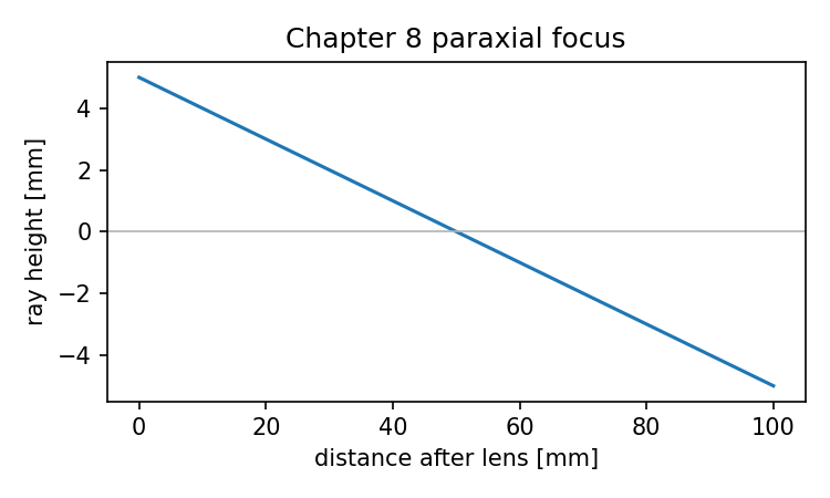
Source and validation note
The ABCD-matrix formulas in this chapter use the sign and ordering conventions stated in the chapter. Other optics books may use different coordinate signs, ray-vector definitions, or multiplication order. When checking results against another source or software package, compare the convention before comparing the number.
Chapter 9: Why Real Rays Depart from Paraxial Rays
A spot diagram is honest, but it is not always explanatory.
It tells you where the rays landed. It shows whether the bundle stayed tight or spread out. It may show a round blur, a comet-like smear, a line, a color separation, or an off-axis distortion. But a spot diagram by itself does not always tell you why the rays landed that way.
To understand why, we need a reference.
Chapter 8 gave us that reference: paraxial optics.
The paraxial model tells us what the optical system does in first order. Near the axis, with small angles, rays behave according to simple linear rules. A field point maps to a paraxial image point. A collimated on-axis bundle focuses at a paraxial focal plane. A thin-lens estimate gives a reasonable scale for focal length. F-number and numerical aperture tell us how wide the ray cone is.
Real rays do not promise to obey that ideal.
They hit the actual surface. They see the exact local normal. They refract by vector Snell’s law. They pass through real thicknesses and real materials. At larger pupil heights and off-axis fields, the exact ray path begins to depart from the paraxial prediction.
That departure is not a vague imperfection.
It can be measured.
This chapter is about measuring and reading that departure.
We will use three ideas:
paraxial reference
real ray intercept
transverse ray error
Then we will turn those errors into ray fan plots and use them to introduce the major aberrations:
spherical aberration
coma
astigmatism
field curvature
distortion
chromatic aberration
We will not do a full third-order aberration derivation. That is a different book. Here, the goal is computational understanding:
Trace the real rays, compare them with a reference, and read the pattern of the error.
This is the gentler path into aberration. Instead of beginning with names, we begin with data.
Aberration is a departure from a reference
The word aberration can sound like a list of named defects you are supposed to memorize.
Spherical aberration. Coma. Astigmatism. Field curvature. Distortion. Chromatic aberration.
Those names matter. Optical designers use them because they describe recognizable patterns. But the names become easier once the underlying idea is clear.
An aberration is a departure from ideal imaging.
For this chapter, we will use a practical ray-based version:
real ray intercept - reference intercept = transverse ray error
If a real ray lands exactly where the reference says it should land, the transverse ray error is zero.
If it lands somewhere else, the error is the difference in image-plane coordinates.
For a ray landing at:
(x_real, y_real)
and a reference point:
(x_ref, y_ref)
the transverse error is:
εx = x_real - x_ref
εy = y_real - y_ref
That is the basic computation behind a ray aberration plot.
The subtle part is not subtraction. The subtle part is choosing the reference.
Common references include:
paraxial image point
chief ray intercept
centroid of the spot
best-focus point
best-fit sphere center, for wavefront-related analysis
Different references answer different questions. If you use the chief ray as the reference, you remove image shift and often remove distortion from the plotted error. If you use the paraxial image point, you can see distortion and field-dependent image displacement. If you use a best-focus reference, you may emphasize residual blur after refocus.
This is why ray fan plots in software are not just “the ray fan.” They are ray fan plots with a reference convention.
We will begin with a simple reference: the chief ray intercept or centroid. Then we will discuss the paraxial reference when distortion matters.
From spot diagram to transverse error
In Chapter 7, our spot diagram points were simply image-plane intercepts:
points = [(x1, y1), (x2, y2), ...]
To convert these into transverse errors, choose a reference.
For a centered spot diagram, we used the centroid:
center = mean(points)
Then:
errors = points - center
That is already a transverse error calculation.
In code:
import numpy as np
import math
import matplotlib.pyplot as plt
def transverse_errors(points, reference=None):
"""Return transverse ray errors relative to a reference point.
points:
Array of shape (N, 2), image-plane x, y intercepts.
reference:
Optional array-like [x_ref, y_ref]. If None, use centroid.
"""
points = np.asarray(points, dtype=float)
if len(points) == 0:
return points, np.array([np.nan, np.nan])
if reference is None:
reference = points.mean(axis=0)
else:
reference = np.asarray(reference, dtype=float)
return points - reference, reference
Use it after collecting spot points:
errors, reference = transverse_errors(spot_points)
print("reference:", reference)
print("first errors:", errors[:5])
If we scatter plot errors[:, 0] and errors[:, 1], we get the centered spot diagram.
But a ray fan does something different.
A ray fan does not only show the two-dimensional distribution of errors. It plots error as a function of pupil coordinate.
That is what makes it diagnostic.
Why ray fans reveal structure
A spot diagram answers:
Where did the rays land?
A ray fan asks:
How does the landing error change as we move across the pupil?
That is a more structured question.
For a tangential fan, we may vary one pupil coordinate across a line:
Px from -1 to +1, Py = 0
Then plot image error against Px.
For a sagittal fan, we vary the other pupil coordinate:
Py from -1 to +1, Px = 0
Then plot image error against Py.
A ray fan is therefore built from line samples through the pupil, not necessarily from a full two-dimensional grid.
This is why ray fans can show aberration patterns more clearly than a dense spot diagram. A spot diagram may look like a cloud. A ray fan shows the functional relationship:
pupil coordinate → transverse error
If the error is mostly a straight line, that often indicates defocus. If it curves with a cubic shape, spherical aberration may be present. If the off-axis fan is asymmetric, coma may be involved. If tangential and sagittal fans behave differently, astigmatism or field curvature may be part of the story.
We will not overclaim from one plot. But we can begin to read the shapes.
Sampling a line across the pupil
Let us create line samples across the pupil.
For an x fan:
x varies from -R to +R
y = 0
For a y fan:
x = 0
y varies from -R to +R
In normalized pupil coordinates, we use:
P = coordinate / pupil_radius
so P runs from -1 to +1.
def sample_pupil_line(axis, num_points, pupil_radius):
"""Sample a line through the circular pupil.
axis:
"x" for x-line samples with y = 0.
"y" for y-line samples with x = 0.
"""
P = np.linspace(-1.0, 1.0, num_points)
points = []
for p in P:
if axis == "x":
points.append((p * pupil_radius, 0.0))
elif axis == "y":
points.append((0.0, p * pupil_radius))
else:
raise ValueError("axis must be 'x' or 'y'")
return P, np.array(points, dtype=float)
We force the number of points to be odd if we want the center ray included:
def odd_count(n):
return n if n % 2 == 1 else n + 1
Now make a line bundle:
def make_line_bundle(
axis,
num_points,
pupil_radius,
z_start,
theta_x_deg=0.0,
theta_y_deg=0.0,
wavelength_um=0.5875618,
):
num_points = odd_count(num_points)
P, pupil_points = sample_pupil_line(axis, num_points, pupil_radius)
rays = make_ray_bundle(
pupil_points=pupil_points,
z_start=z_start,
theta_x_deg=theta_x_deg,
theta_y_deg=theta_y_deg,
wavelength_um=wavelength_um,
)
return P, rays
This gives us both the normalized pupil coordinates and the rays.
Building a ray fan from our singlet tracer
We can now trace a line bundle through the simple singlet from the previous chapters.
Assume we still have:
front
back
image
N_BK7
trace_bundle_through_singlet(...)
collect_image_points(...)
Now write a ray fan function.
def ray_fan_for_singlet(
axis,
num_points,
pupil_radius,
z_start,
theta_x_deg,
theta_y_deg,
wavelength_um,
front,
back,
image,
glass_material,
reference="centroid",
):
"""Compute a simple transverse ray fan for the singlet.
Returns:
P: normalized pupil coordinates
errors: transverse errors, shape (N, 2), for valid rays
points: image-plane intercepts
valid_mask: Boolean mask for rays that reached the image plane
ref: reference point used for transverse error
"""
P, rays = make_line_bundle(
axis=axis,
num_points=num_points,
pupil_radius=pupil_radius,
z_start=z_start,
theta_x_deg=theta_x_deg,
theta_y_deg=theta_y_deg,
wavelength_um=wavelength_um,
)
traced = trace_bundle_through_singlet(
rays,
front=front,
back=back,
image=image,
glass_material=glass_material,
)
points = []
valid_P = []
for p, ray in zip(P, traced):
if ray.alive:
points.append((ray.position[0], ray.position[1]))
valid_P.append(p)
points = np.array(points, dtype=float)
valid_P = np.array(valid_P, dtype=float)
if len(points) == 0:
return valid_P, points, points, np.array([], dtype=bool), np.array([np.nan, np.nan])
if reference == "centroid":
errors, ref = transverse_errors(points)
elif reference == "chief":
# With odd line sampling, the center point is the closest chief-like sample
center_index = np.argmin(np.abs(valid_P))
ref = points[center_index]
errors, ref = transverse_errors(points, reference=ref)
else:
raise ValueError("reference must be 'centroid' or 'chief'")
return valid_P, errors, points, ref
Now plot the fan.
For an on-axis field, use an x fan:
P, errors, points, ref = ray_fan_for_singlet(
axis="x",
num_points=51,
pupil_radius=5.0,
z_start=-20.0,
theta_x_deg=0.0,
theta_y_deg=0.0,
wavelength_um=0.5875618,
front=front,
back=back,
image=image,
glass_material=N_BK7,
reference="chief",
)
plt.plot(P, errors[:, 0], marker=".")
plt.axhline(0.0, linewidth=0.8)
plt.axvline(0.0, linewidth=0.8)
plt.xlabel("normalized pupil coordinate P_x")
plt.ylabel("transverse error εx [mm]")
plt.title("On-axis x ray fan")
plt.show()
That plot is a ray fan.
It is not a new kind of physics. It is a different organization of the same traced ray data.
ray trace → image intercepts → subtract reference → plot error versus pupil coordinate
That is the whole construction.
Defocus: the simplest ray fan shape
Before naming complicated aberrations, start with defocus.
Suppose a bundle would ideally focus at one plane, but we measure it at a plane before or after focus. Then ray intercepts shift roughly linearly with pupil coordinate. Edge rays land on one side, center rays near the reference, opposite edge rays on the other side.
The ray fan becomes approximately a straight line.
This is easy to simulate by moving the image plane.
def make_image_plane(z_image):
return IntersectableSurface(
radius=float("inf"),
z_vertex=z_image,
semi_diameter=None,
surface_type="plane",
comment="image plane",
)
Now compare fans at different image positions:
for z_image in [40.0, 50.0, 60.0]:
image_test = make_image_plane(z_image)
P, errors, points, ref = ray_fan_for_singlet(
axis="x",
num_points=51,
pupil_radius=5.0,
z_start=-20.0,
theta_x_deg=0.0,
theta_y_deg=0.0,
wavelength_um=0.5875618,
front=front,
back=back,
image=image_test,
glass_material=N_BK7,
reference="chief",
)
plt.plot(P, errors[:, 0], marker=".", label=f"z={z_image:.0f} mm")
plt.axhline(0.0, linewidth=0.8)
plt.axvline(0.0, linewidth=0.8)
plt.xlabel("normalized pupil coordinate P_x")
plt.ylabel("transverse error εx [mm]")
plt.title("Defocus changes the slope of the ray fan")
plt.legend()
plt.show()
The main change is often a linear tilt in the fan.
This is useful because defocus can mask other patterns. If the image plane is not at a meaningful focus, the ray fan may be dominated by a straight-line term. Once you refocus, the residual curvature becomes easier to inspect.
This is why optical analysis software often lets you change focus or subtract certain reference terms. The plot is not just a raw truth. It is a diagnostic view.
Spherical aberration: edge rays do not focus like near-axis rays
Spherical aberration is one of the most natural aberrations to see with our current code.
For an on-axis object point, a perfect paraxial model would bring all incoming parallel rays to the same focus. A real spherical surface does not generally do that. Rays hitting the lens near the edge may cross the axis at a different z position than rays near the center.
In a ray fan, spherical aberration often appears as a curved pattern, commonly with a cubic-like shape in transverse ray error versus pupil coordinate.
Let us compute approximate axis crossing after the singlet for different input heights.
def trace_simple_singlet_to_exit(ray, front, back, glass_material):
n_air = 1.0
n_glass = glass_material.n(ray.wavelength_um)
interact_refractive_surface(ray, front, n1=n_air, n2=n_glass)
if ray.alive:
interact_refractive_surface(ray, back, n1=n_glass, n2=n_air)
return ray
def z_axis_crossing_xz(ray):
"""Estimate where a ray in the x-z plane crosses x=0 after exit."""
x0 = ray.position[0]
z0 = ray.position[2]
dx = ray.direction[0]
dz = ray.direction[2]
if abs(dx) < 1e-12:
return math.inf
t = -x0 / dx
if t < 0:
return math.inf
return z0 + t * dz
Now sweep ray height:
heights = np.linspace(0.5, 8.0, 16)
crossings = []
for h in heights:
ray = Ray(
position=[h, 0.0, -20.0],
direction=[0.0, 0.0, 1.0],
wavelength_um=0.5875618,
)
trace_simple_singlet_to_exit(ray, front, back, N_BK7)
crossings.append(z_axis_crossing_xz(ray))
plt.plot(heights, crossings, marker=".")
plt.xlabel("input ray height [mm]")
plt.ylabel("axis crossing z [mm]")
plt.title("Longitudinal focus shift with ray height")
plt.show()
If the crossing position changes with ray height, the lens has spherical aberration under this setup.
That statement is not a label pulled from memory. It follows from the data:
near-axis rays focus here
edge rays focus somewhere else
This is spherical aberration in computational form.
Transverse spherical aberration at a fixed image plane
Axis crossing is a longitudinal view. A ray fan at a fixed image plane gives a transverse view.
Pick an image plane. Trace rays across the pupil. Plot transverse error.
image_focus = make_image_plane(50.0)
P, errors, points, ref = ray_fan_for_singlet(
axis="x",
num_points=101,
pupil_radius=5.0,
z_start=-20.0,
theta_x_deg=0.0,
theta_y_deg=0.0,
wavelength_um=0.5875618,
front=front,
back=back,
image=image_focus,
glass_material=N_BK7,
reference="chief",
)
plt.plot(P, errors[:, 0])
plt.axhline(0.0, linewidth=0.8)
plt.axvline(0.0, linewidth=0.8)
plt.xlabel("normalized pupil coordinate P_x")
plt.ylabel("transverse error εx [mm]")
plt.title("On-axis transverse ray fan")
plt.show()
For a rotationally symmetric on-axis system, the x fan and y fan should behave similarly. If the plot is curved and symmetric in the expected way, you are seeing how ray height changes focus and image-plane intercept.
Do not worry about naming every coefficient. The computational interpretation is enough:
the error is not constant
the error is not only a linear defocus term
the error varies with pupil coordinate
That variation is the ray trace exposing aberration.
Coma: off-axis asymmetry
Now move off-axis.
Coma appears for off-axis field points when rays from different pupil zones produce an asymmetric blur. In a spot diagram, coma can look like a comet: a dense head and a spreading tail. In ray fan plots, coma introduces asymmetric terms that are not present for the on-axis symmetric case.
Let us trace an off-axis field:
image_focus = make_image_plane(50.0)
P, errors, points, ref = ray_fan_for_singlet(
axis="y",
num_points=101,
pupil_radius=5.0,
z_start=-20.0,
theta_x_deg=0.0,
theta_y_deg=5.0,
wavelength_um=0.5875618,
front=front,
back=back,
image=image_focus,
glass_material=N_BK7,
reference="chief",
)
plt.plot(P, errors[:, 1])
plt.axhline(0.0, linewidth=0.8)
plt.axvline(0.0, linewidth=0.8)
plt.xlabel("normalized pupil coordinate P_y")
plt.ylabel("transverse error εy [mm]")
plt.title("Off-axis ray fan")
plt.show()
Now also plot the off-axis spot:
pupil_points = sample_pupil_grid(samples_per_axis=17, pupil_radius=5.0)
rays = make_ray_bundle(
pupil_points=pupil_points,
z_start=-20.0,
theta_x_deg=0.0,
theta_y_deg=5.0,
wavelength_um=0.5875618,
)
traced = trace_bundle_through_singlet(rays, front, back, image_focus, N_BK7)
spot_points, valid = collect_image_points(traced)
spot_errors, ref = transverse_errors(spot_points)
plot_spot(spot_errors, title="Off-axis spot, centered")
If the centered spot is asymmetric, that is a clue. If the ray fan shows asymmetric departure as pupil coordinate changes, that is another clue.
This is the practical way to meet coma:
not as a word first,
but as an off-axis asymmetric error pattern in traced ray data.
A simple singlet is not corrected for off-axis aberrations, so it is a good teaching object. It behaves badly enough to show the problem.
Tangential and sagittal behavior
Off-axis systems have a special complication.
There are two important planes:
tangential plane
sagittal plane
If the field is in the y direction, the tangential plane contains the optical axis and the field direction. The sagittal plane is perpendicular to it.
In practical ray fan terms, we often inspect two fans:
tangential fan
sagittal fan
The exact naming depends on coordinate convention. The important computational idea is:
Sample rays along two orthogonal pupil lines and compare their transverse errors.
If the tangential and sagittal fans behave differently, the system is telling you that off-axis imaging is not the same in the two planes.
That difference is connected to astigmatism and field curvature.
Let us compute both line fans for the same off-axis field:
field_angle = 5.0
image_focus = make_image_plane(50.0)
P_x, errors_x, points_x, ref_x = ray_fan_for_singlet(
axis="x",
num_points=101,
pupil_radius=5.0,
z_start=-20.0,
theta_x_deg=0.0,
theta_y_deg=field_angle,
wavelength_um=0.5875618,
front=front,
back=back,
image=image_focus,
glass_material=N_BK7,
reference="chief",
)
P_y, errors_y, points_y, ref_y = ray_fan_for_singlet(
axis="y",
num_points=101,
pupil_radius=5.0,
z_start=-20.0,
theta_x_deg=0.0,
theta_y_deg=field_angle,
wavelength_um=0.5875618,
front=front,
back=back,
image=image_focus,
glass_material=N_BK7,
reference="chief",
)
plt.plot(P_x, errors_x[:, 0], label="x fan: εx")
plt.plot(P_y, errors_y[:, 1], label="y fan: εy")
plt.axhline(0.0, linewidth=0.8)
plt.axvline(0.0, linewidth=0.8)
plt.xlabel("normalized pupil coordinate")
plt.ylabel("transverse error [mm]")
plt.title("Two orthogonal ray fans for an off-axis field")
plt.legend()
plt.show()
This comparison is more informative than either curve alone.
If one plane focuses differently from the other, moving the image plane may improve one fan while worsening the other. That is the practical sign of astigmatic behavior.
Astigmatism: two line foci instead of one point focus
Astigmatism does not mean “everything is blurry” in a generic way.
For an off-axis field, rays in two orthogonal sections of the bundle may come to best focus at different axial positions. Instead of one clean point focus, the system has two preferred line-like foci: tangential and sagittal.
A simple way to see this computationally is to scan image plane position and compute RMS width in two directions.
Let us use off-axis ray bundles and measure spot spread as the image plane moves.
def spot_statistics_for_plane(z_image, field_angle, wavelength_um=0.5875618):
image_test = make_image_plane(z_image)
pupil_points = sample_pupil_grid(samples_per_axis=17, pupil_radius=5.0)
rays = make_ray_bundle(
pupil_points=pupil_points,
z_start=-20.0,
theta_x_deg=0.0,
theta_y_deg=field_angle,
wavelength_um=wavelength_um,
)
traced = trace_bundle_through_singlet(rays, front, back, image_test, N_BK7)
points, valid = collect_image_points(traced)
if len(points) == 0:
return np.nan, np.nan, np.nan
centered, ref = transverse_errors(points)
rms_x = math.sqrt(float(np.mean(centered[:, 0]**2)))
rms_y = math.sqrt(float(np.mean(centered[:, 1]**2)))
rms_r = rms_spot_radius(points)
return rms_x, rms_y, rms_r
Sweep focus:
z_values = np.linspace(35.0, 70.0, 71)
field_angle = 5.0
rms_x_values = []
rms_y_values = []
rms_r_values = []
for z in z_values:
rms_x, rms_y, rms_r = spot_statistics_for_plane(z, field_angle)
rms_x_values.append(rms_x)
rms_y_values.append(rms_y)
rms_r_values.append(rms_r)
plt.plot(z_values, rms_x_values, label="RMS x")
plt.plot(z_values, rms_y_values, label="RMS y")
plt.plot(z_values, rms_r_values, label="RMS radius")
plt.xlabel("image plane z [mm]")
plt.ylabel("RMS spot size [mm]")
plt.title("Focus scan for an off-axis field")
plt.legend()
plt.show()
If the minima of RMS x and RMS y occur at different z positions, the system has different best focus behavior in two transverse directions.
That is the computational flavor of astigmatism.
Again, we are not asking you to memorize a diagram. We are showing how a ray trace reveals the effect.
Field curvature: best focus changes across the field
A flat sensor is flat. Real optical systems may prefer a curved image surface.
Field curvature means that the best focus position changes with field. The center field might focus at one image plane, while the edge field wants another.
This is easy to confuse with ordinary defocus unless you compare multiple field points.
Let us compute the best RMS focus for several fields.
def best_focus_by_rms(field_angle, z_min=35.0, z_max=70.0, count=71):
z_values = np.linspace(z_min, z_max, count)
rms_values = []
for z in z_values:
_, _, rms_r = spot_statistics_for_plane(z, field_angle)
rms_values.append(rms_r)
rms_values = np.array(rms_values)
idx = np.nanargmin(rms_values)
return z_values[idx], rms_values[idx], z_values, rms_values
Run it:
for field_angle in [0.0, 2.0, 4.0, 6.0]:
z_best, rms_best, _, _ = best_focus_by_rms(field_angle)
print(
f"field={field_angle:.1f} deg, "
f"best z≈{z_best:.2f} mm, "
f"best RMS≈{rms_best:.6f} mm"
)
If best focus shifts with field, that is field curvature in computational terms.
A flat image plane cannot satisfy every field perfectly if the best-focus surface is curved. A designer may accept this, correct it, or balance it against other aberrations. A camera lens, microscope objective, eyepiece, or projection lens may care about this differently.
The key point is simple:
field curvature is not just blur at the edge.
It is a field-dependent best-focus position.
A focus scan makes that visible.
Distortion: image position is wrong even if the spot is sharp
Distortion is different from blur.
A lens can form a relatively sharp image point at the wrong location. That is distortion.
This is why a centered spot diagram can hide distortion. If you subtract the centroid or chief ray intercept, you remove the image displacement and look only at spread. That is useful for blur, but not for mapping accuracy.
To see distortion, compare real image height with paraxial image height.
From Chapter 8:
y_paraxial ≈ f tan θ
For our simple singlet, we can use a thin-lens focal length estimate as a rough reference. A real library’s paraxial analysis would give a better reference from the actual prescription, but the thin-lens estimate is enough to show the method.
def real_chief_ray_image_height(field_angle_deg, z_image, wavelength_um=0.5875618):
image_test = make_image_plane(z_image)
chief = make_chief_ray(
z_start=-20.0,
theta_x_deg=0.0,
theta_y_deg=field_angle_deg,
wavelength_um=wavelength_um,
)
trace_simple_singlet_ray(chief, front, back, image_test, N_BK7)
if not chief.alive:
return np.nan
return chief.position[1]
Now compare:
f_est = thin_lens_focal_length_from_radii(
N_BK7.n(0.5875618),
R1=50.0,
R2=-50.0,
)
z_image = 50.0
for field_angle in [1.0, 2.0, 3.0, 5.0, 7.0]:
y_real = real_chief_ray_image_height(field_angle, z_image)
y_para = paraxial_image_height_from_field(f_est, field_angle)
error = y_real - y_para
print(
f"field={field_angle:.1f} deg, "
f"real y={y_real:.4f} mm, "
f"paraxial y={y_para:.4f} mm, "
f"distortion-like error={error:.4f} mm"
)
This is not a polished distortion analysis. The focal length reference is crude, and our simple chief ray model is simplified. But the structure is correct:
field angle
→ paraxial image height
→ real chief ray image height
→ difference
That difference is mapping error.
The spot could be tiny and the mapping could still be distorted. That is why distortion belongs in the aberration family but behaves differently from blur.
Chromatic aberration: different wavelengths, different rays
Chromatic aberration comes from the material model.
In Chapter 3, we learned that glass refractive index depends on wavelength:
n = n(λ)
In Chapter 6, we used that index in Snell’s law.
Therefore rays of different wavelengths do not trace exactly the same path through the same lens.
There are two common chromatic effects to notice:
longitudinal chromatic aberration:
different wavelengths focus at different axial positions
lateral chromatic aberration:
different wavelengths have different image heights off-axis
Let us compute a simple longitudinal chromatic focus estimate.
for wl in [0.4861327, 0.5875618, 0.6562725]:
z_best, rms_best, _, _ = best_focus_by_rms(
field_angle=0.0,
z_min=35.0,
z_max=70.0,
count=71,
)
print(wl, z_best, rms_best)
This version accidentally uses the default wavelength inside spot_statistics_for_plane, so let us make the wavelength explicit.
def best_focus_by_rms_for_wavelength(
field_angle,
wavelength_um,
z_min=35.0,
z_max=70.0,
count=71,
):
z_values = np.linspace(z_min, z_max, count)
rms_values = []
for z in z_values:
rms_x, rms_y, rms_r = spot_statistics_for_plane(
z_image=z,
field_angle=field_angle,
wavelength_um=wavelength_um,
)
rms_values.append(rms_r)
rms_values = np.array(rms_values)
idx = np.nanargmin(rms_values)
return z_values[idx], rms_values[idx]
Now compute:
for wl in [0.4861327, 0.5875618, 0.6562725]:
z_best, rms_best = best_focus_by_rms_for_wavelength(
field_angle=0.0,
wavelength_um=wl,
)
print(
f"λ={wl:.7f} µm, "
f"best focus z≈{z_best:.2f} mm, "
f"best RMS≈{rms_best:.6f} mm"
)
If the best focus differs by wavelength, you are seeing longitudinal chromatic aberration.
For lateral chromatic aberration, compare off-axis chief ray image heights by wavelength:
field_angle = 5.0
z_image = 50.0
for wl in [0.4861327, 0.5875618, 0.6562725]:
y_real = real_chief_ray_image_height(
field_angle_deg=field_angle,
z_image=z_image,
wavelength_um=wl,
)
print(f"λ={wl:.7f} µm, chief ray image y={y_real:.6f} mm")
If image height changes with wavelength, that is lateral color in this simplified analysis.
The singlet is not meant to look good. It will not. It is useful because chromatic aberration emerges from the same ray-tracing machinery.
No special “chromatic aberration module” is needed at the conceptual level.
The chain is:
wavelength
→ refractive index
→ refracted direction
→ image intercept
→ wavelength-dependent focus or image height
A taxonomy from computations, not from memorization
Now we can summarize the classical aberrations in computational terms.
Spherical aberration
On-axis rays at different pupil radii focus differently.
Computational sign:
axis crossing z changes with pupil height
on-axis ray fan shows curved error versus pupil coordinate
Coma
Off-axis rays form an asymmetric blur.
Computational sign:
off-axis spot becomes asymmetric
off-axis ray fan shows asymmetric error terms
Astigmatism
Tangential and sagittal sections focus differently.
Computational sign:
two orthogonal fan directions behave differently
RMS x and RMS y may have minima at different image planes
Field curvature
Best focus changes with field.
Computational sign:
best RMS focus z shifts as field angle changes
flat image plane cannot match all fields equally
Distortion
Image point is displaced from the paraxial mapping, even if the spot is sharp.
Computational sign:
real chief ray or centroid image height differs from paraxial image height
centered spot diagram may hide it
Chromatic aberration
Different wavelengths image differently.
Computational sign:
best focus shifts with wavelength
off-axis image height changes with wavelength
polychromatic spot separates by color
This way of learning aberrations is slower than memorizing a table. It is also sturdier.
The names now attach to measured behavior.
Why real ray fans are not wavefront maps
A ray fan plot is powerful, but it is still ray-based.
It plots transverse image error versus pupil coordinate. It does not directly show optical path difference. It does not by itself give PSF or MTF. It is still part of geometric optics.
That limitation matters.
Two systems with similar spot diagrams may have different wavefront phase behavior. Diffraction can dominate when geometric spots become small. A lens near diffraction-limited performance needs wavefront analysis, not only ray intercepts.
So this chapter is a bridge, but not the final bridge.
We have moved from:
where do rays land?
to:
how do real rays depart from a reference?
The next chapter moves to:
how do ray paths become optical path difference across the pupil?
That is the bridge from geometric ray tracing to wave optics.
Optiland RayFan as a higher-level version
A real optical library already has ray fan tools.
In current Optiland documentation, the RayFan analysis takes an optic, fields, wavelengths, and a number of points; it traces line distributions across the pupil and stores x and y ray fan data. The source also shows that the standard view plots ray fan error against normalized pupil coordinates, with separate x and y fan panels. (Optiland)
A compact Optiland-style workflow looks like this:
from optiland.samples.objectives import CookeTriplet
from optiland.analysis import RayFan
lens = CookeTriplet()
fan = RayFan(
lens,
fields="all",
wavelengths="all",
num_points=101,
)
fan.view()
For a custom singlet, the setup would follow the same optical-system construction style used earlier:
from optiland import optic
from optiland.analysis import RayFan
lens = optic.Optic()
lens.surfaces.add(index=0, radius=float("inf"), thickness=float("inf"))
lens.surfaces.add(index=1, radius=50.0, thickness=5.0, material="N-BK7", is_stop=True)
lens.surfaces.add(index=2, radius=-50.0, thickness=45.0)
lens.surfaces.add(index=3)
lens.set_aperture(aperture_type="EPD", value=10.0)
lens.fields.set_type("angle")
lens.fields.add(y=0.0)
lens.fields.add(y=5.0)
lens.wavelengths.add(value=0.5876, is_primary=True)
fan = RayFan(lens, fields="all", wavelengths="all", num_points=101)
fan.view()
Treat this as library-level comparison code. Exact import paths and options can change as the project evolves, but the computational meaning is stable:
select field and wavelength
trace line samples through the pupil
measure image-plane transverse error
plot error versus normalized pupil coordinate
The current Optiland source also includes a BestFitRayFan class that references ray fan data to a best-fit sphere center rather than the ordinary chief-ray-centered reference. That is a useful reminder that ray fan plots depend on reference convention, not only on traced rays. (Optiland)
This is exactly why we built the small version ourselves first.
When a library gives you a beautiful fan plot, you can now ask:
What pupil line was sampled?
What field and wavelength were used?
What reference point was subtracted?
Was distortion removed?
Were invalid rays suppressed?
Those questions are not pedantic. They determine what the plot means.
A small diagnostic workflow
When reading ray fan results, use a disciplined order.
First, check the setup:
field
wavelength
aperture
image plane
reference convention
sampling density
Second, check whether rays were lost:
blocked by aperture
missed a surface
total internal reflection
invalid image intercept
Third, separate defocus from residual shape. If the fan is mostly a straight line, move the image plane or subtract focus before diagnosing more subtle aberrations.
Fourth, compare x and y fans. Do not assume one fan tells the full story.
Fifth, compare fields. On-axis and off-axis behavior are often completely different.
Sixth, compare wavelengths. If the curves separate by wavelength, the material model is speaking.
Finally, connect the fan to the spot diagram. The fan explains structure. The spot shows the two-dimensional landing pattern. Neither replaces the other.
This workflow is more reliable than trying to recognize every aberration by visual memory alone.
Common mistakes when interpreting aberrations
Let us name the traps clearly.
Mistake 1: Calling every blur “spherical aberration”
Spherical aberration is specifically about how ray behavior changes with pupil radius for an on-axis field. Off-axis blur may involve coma, astigmatism, field curvature, and other effects.
Mistake 2: Forgetting the image plane
A ray fan can be dominated by defocus if the image plane is poorly chosen. Before diagnosing subtle aberrations, check focus.
Mistake 3: Centering away distortion
A centered spot or chief-ray-referenced fan may remove image displacement. That is useful for blur analysis, but it can hide distortion.
Mistake 4: Comparing fans with different references
A fan referenced to the chief ray is not the same as a fan referenced to a paraxial image point or best-fit focus.
Mistake 5: Ignoring wavelength
A monochromatic fan cannot show chromatic separation. A polychromatic fan may contain several overlapping stories.
Mistake 6: Reading a sparse fan too confidently
Sampling density matters. Too few points can hide curvature or make a curve look cleaner than it is.
Mistake 7: Treating ray fans as diffraction analysis
Ray fans are geometric. They do not directly tell you the diffraction PSF or MTF.
Mistake 8: Forgetting units
A fan error of 0.01 mm may be large or small depending on pixel size, Airy disk size, focal length, and intended use.
Mistake 9: Expecting a simple singlet to behave like a corrected objective
A biconvex singlet is a teaching system. It will show aberrations clearly because it is not corrected. That is useful here.
Mistake 10: Diagnosing from one plot alone
Use spot diagrams, ray fans, focus scans, field comparisons, and wavelength comparisons together. One plot rarely tells the whole truth.
What this chapter gives us
We now have a computational way to discuss aberration.
We can:
trace real rays through a lens
choose a reference intercept
compute transverse ray error
sample line fans across the pupil
plot ray fan curves
scan focus position
compare fields
compare wavelengths
connect ray fan shapes to classical aberrations
The important shift is this:
Aberrations are no longer just names. They are patterns in computed ray error.
This is the right level of understanding for the rest of the book.
When we later compute OPD, PSF, OTF, and MTF, we will not forget the ray story. Wave optics does not erase geometric optics. It extends it. The wavefront across the pupil is built from optical path differences, and those paths come from traced rays through the system.
Ray fans tell us how rays miss.
Wavefront maps will tell us how phase departs.
PSF will show how a point spreads.
MTF will show how contrast survives.
The chain is getting longer, but each link is now visible.
The road ahead
The ray fan is a powerful diagnostic, but it still lives in image-plane coordinates. It tells us transverse error.
To reach diffraction analysis, we need a different quantity.
We need optical path difference.
A ray does not only land somewhere. It also accumulates optical path length as it travels through air and glass. Different rays across the pupil may arrive with different optical path lengths relative to a reference wavefront. That difference becomes phase error.
That is the bridge from ray tracing to wave optics.
The next chapter will therefore ask:
How do we turn traced ray paths into OPD across the pupil?
Once we have OPD, the later chapters can build the pupil function, PSF, OTF, and finally MTF.
A spot diagram comes from where rays land.
A wavefront map comes from how much optical path they carry.
We now know the first. Next, we learn the second.
Generated validation figure
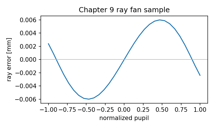
Chapter 10: OPD and Wavefront Error
A spot diagram tells us where rays land.
That is useful. Very useful. In Chapter 7, the spot diagram was our first real analysis plot. In Chapter 9, ray fans helped us see how real rays depart from a paraxial reference. We could look at transverse ray error and begin to recognize spherical aberration, coma, astigmatism, field curvature, distortion, and chromatic effects.
But there is a limit to this way of looking.
A ray can land near the right place and still arrive with the wrong phase.
That sentence is the doorway to the next part of the book.
Geometric ray tracing tracks where rays go. Diffraction imaging cares about how the optical field adds up. To compute a PSF by Fourier methods, we need not only a collection of ray intercepts. We need a complex pupil function. To build that pupil function, we need phase across the pupil. To get phase, we need optical path difference.
That is the bridge:
real ray tracing
→ optical path length
→ optical path difference
→ wavefront error
→ pupil phase
→ PSF
→ OTF
→ MTF
This chapter is about the middle of that bridge.
We will ask:
What is optical path length?
What is OPD?
What is the reference wavefront?
Why is OPD usually shown over the pupil?
How can we create a simple OPD map in Python?
How does this connect to Optiland wavefront analysis?
We will not compute a production-quality OPD from a full ray trace in this chapter. That requires careful reference geometry, exit pupil coordinates, ray aiming, focus conventions, and surface-by-surface optical path bookkeeping. A real library handles those details. Current Optiland wavefront tools, for example, include OPD and wavefront analysis modules, and its Wavefront class is documented as computing exit-pupil ray intersections, OPD, ray intensities, and reference-sphere radius according to selected strategies. (Optiland)
Our job here is to understand what those tools are calculating.
So we will do two things:
1. Build the concept carefully.
2. Generate simplified OPD maps ourselves.
Once you understand the OPD map, Chapter 11 can turn it into a complex pupil function.
That is the moment geometric optics becomes Fourier optics.
Why ray landing points are not enough
Imagine two rays that reach the same point on the image plane.
From a spot diagram alone, they look perfect. They landed together.
But suppose one ray has traveled a slightly longer optical path than the other. Then their phases may not match when the waves interfere. If the phase difference is small, they add mostly constructively. If the phase difference is large, they may partially cancel or create structure in the diffraction pattern.
A spot diagram cannot show that.
A spot diagram records transverse position:
x_image, y_image
A wavefront analysis records optical path difference across the pupil:
OPD(Px, Py)
These are different kinds of data.
Ray intercepts answer:
Where did the rays go?
OPD answers:
How much optical phase delay does each pupil point carry relative to a reference?
Both matter.
For a badly aberrated lens, spot diagrams can be very informative. For a nearly diffraction-limited lens, spot diagrams may become less revealing. The geometric spot may be tiny, but the wavefront phase still determines the detailed diffraction pattern.
That is why we need OPD.
It is the missing quantity between ray tracing and PSF.
Optical path length
A ray traveling through air and glass does not only cover geometric distance. It accumulates optical path length.
For a small segment of length ds in a medium of refractive index n, the optical path contribution is:
dOPL = n ds
Along a full path:
OPL = ∫ n ds
In a ray tracer with discrete segments, this becomes:
OPL = n1 s1 + n2 s2 + n3 s3 + ...
where:
s1, s2, s3 = geometric segment lengths
n1, n2, n3 = refractive indices along those segments
This is why our Ray class has carried opl since Chapter 4.
When we wrote:
ray.propagate(distance, refractive_index=n)
we updated:
ray.opl += n * distance
At the time, that may have looked like extra bookkeeping. Now it becomes essential.
The ray’s final position tells us where it landed.
The ray’s accumulated OPL tells us how much optical distance it traveled.
Those two pieces of information lead to different analyses.
A tiny OPL example
Let us revisit the simplest possible path.
A ray travels:
20 mm in air
5 mm in glass
20 mm in air
If the glass index is 1.5, then:
geometric distance = 20 + 5 + 20 = 45 mm
OPL = 1.0×20 + 1.5×5 + 1.0×20 = 47.5 mm
In code:
segments = [
{"distance_mm": 20.0, "n": 1.0},
{"distance_mm": 5.0, "n": 1.5},
{"distance_mm": 20.0, "n": 1.0},
]
opl = sum(seg["distance_mm"] * seg["n"] for seg in segments)
geometric = sum(seg["distance_mm"] for seg in segments)
print("geometric distance [mm]:", geometric)
print("optical path length [mm]:", opl)
The ray has physically traveled 45 mm, but optically it has traveled 47.5 mm.
This difference is not cosmetic. It determines phase.
If another ray travels a slightly different optical path, the two rays may arrive with different phase even if their geometric endpoints are close.
From OPL to OPD
Optical path length by itself is not yet wavefront error.
OPL is an absolute accumulated path along one ray. OPD is a difference relative to a reference.
A simple definition is:
OPD = OPL_ray - OPL_reference
But the reference matters.
For imaging, the ideal reference is usually not a flat plane. A perfect converging wave heading toward an image point has a spherical wavefront centered on that image point. So the reference wavefront is often a sphere.
That means OPD is more carefully understood as:
the optical path difference between the actual wavefront and a chosen reference wavefront
or, in ray terms:
how much each ray's optical path differs from the ideal reference path
This is where wavefront analysis becomes a little subtle. We must decide what “ideal” means.
Possible reference choices include:
chief-ray reference sphere
centroid-based reference sphere
best-fit reference sphere
paraxial reference sphere
image-plane reference
Different choices remove or retain different low-order terms such as piston, tilt, and defocus. This is not cheating. It is choosing what question the OPD map should answer.
Current Optiland documentation reflects this idea directly: its Wavefront analysis accepts strategy choices such as chief_ray, centroid_sphere, and best_fit_sphere, and includes a remove_tilt option for OPD data. (Optiland)
That tells us something important:
OPD is not only a raw number. It is a number relative to a reference geometry.
The reference must be known before the OPD map can be interpreted.
OPD in length and OPD in waves
OPD can be expressed in length units:
OPD = 0.00025 mm
It can also be expressed in waves:
OPD_waves = OPD_length / wavelength
This is often more useful for phase.
If the wavelength is 0.5 µm, then an OPD of 0.25 µm is half a wave:
0.25 µm / 0.5 µm = 0.5 waves
Phase is related to OPD in waves by:
phase = 2π × OPD_waves
or, using length units:
phase = 2π × OPD_length / wavelength
This unit conversion is a place where mistakes love to hide.
If OPL is stored in millimeters and wavelength is stored in micrometers, we must convert:
wavelength_mm = wavelength_um × 1e-3
Then:
OPD_waves = OPD_mm / wavelength_mm
Let us write helpers:
import numpy as np
import math
import matplotlib.pyplot as plt
def wavelength_um_to_mm(wavelength_um):
return wavelength_um * 1e-3
def opd_mm_to_waves(opd_mm, wavelength_um):
wavelength_mm = wavelength_um_to_mm(wavelength_um)
return opd_mm / wavelength_mm
def opd_waves_to_phase(opd_waves):
return 2.0 * np.pi * opd_waves
Test:
opd_um = 0.25
wavelength_um = 0.5
opd_mm = opd_um * 1e-3
waves = opd_mm_to_waves(opd_mm, wavelength_um)
print("OPD [waves]:", waves)
print("phase [radians]:", opd_waves_to_phase(waves))
The result should be:
0.5 waves
π radians
This is the step that Chapter 11 will use directly.
Pupil coordinates
OPD is usually shown as a function over the pupil.
Instead of plotting OPD versus image-plane coordinates, we plot it over normalized pupil coordinates:
Px, Py
where the pupil circle is:
Px² + Py² <= 1
A pupil coordinate identifies where a sampled ray passes through the pupil. For each point in the pupil, the wavefront has some optical path difference relative to the reference.
So an OPD map is:
OPD(Px, Py)
This is why wavefront maps look like colored disks. The disk is the pupil. The color is OPD.
Let us create a pupil grid.
def make_normalized_pupil_grid(N):
"""Create a square grid with a circular pupil mask.
Returns
-------
X, Y:
Meshgrid coordinates from -1 to +1.
R:
Radius sqrt(X^2 + Y^2).
mask:
Boolean circular aperture mask.
"""
u = np.linspace(-1.0, 1.0, N)
X, Y = np.meshgrid(u, u)
R = np.sqrt(X**2 + Y**2)
mask = R <= 1.0
return X, Y, R, mask
Plot the mask:
X, Y, R, mask = make_normalized_pupil_grid(256)
plt.imshow(mask, extent=[-1, 1, -1, 1], origin="lower")
plt.xlabel("Pupil X")
plt.ylabel("Pupil Y")
plt.title("Circular pupil mask")
plt.colorbar(label="inside pupil")
plt.show()
This is not yet OPD. It is the domain where OPD will live.
A simplified wavefront function
Now we will generate an OPD map directly.
This is not yet computed from a full ray trace. It is a controlled teaching model. We choose a wavefront error function over the pupil, then visualize it.
This is useful because the goal of this chapter is representation:
OPD over pupil → phase → pupil function
The source of the OPD can be a real ray trace, a fitted Zernike model, a measured wavefront sensor, or a simplified polynomial. The representation is the same.
Let us build a toy wavefront in waves.
Use normalized pupil coordinates:
X, Y ∈ [-1, 1]
R² = X² + Y²
Add simple terms:
defocus-like term: 2R² - 1
astigmatism-like term: X² - Y²
coma-like term: (3R² - 2)Y
spherical-like term: 6R⁴ - 6R² + 1
These are not carefully normalized Zernike polynomials. They are teaching shapes. That is enough for seeing how OPD maps work.
def toy_opd_waves(X, Y, mask, defocus=0.0, astig=0.0, coma=0.0, spherical=0.0):
"""Create a toy OPD map in waves over a normalized circular pupil.
The terms are simple teaching polynomials, not normalized Zernikes.
"""
R2 = X**2 + Y**2
R4 = R2**2
W = np.zeros_like(X, dtype=float)
W += defocus * (2.0 * R2 - 1.0)
W += astig * (X**2 - Y**2)
W += coma * (3.0 * R2 - 2.0) * Y
W += spherical * (6.0 * R4 - 6.0 * R2 + 1.0)
W = np.where(mask, W, np.nan)
return W
Now create a map:
X, Y, R, mask = make_normalized_pupil_grid(256)
W = toy_opd_waves(
X, Y, mask,
defocus=0.25,
astig=0.10,
coma=0.08,
spherical=0.05,
)
Here W is OPD in waves.
That means:
W = 1.0 means one wavelength of OPD
W = 0.5 means half a wavelength
W = 0.0 means equal to the reference
Plot it:
def plot_opd_map(W, title="OPD map [waves]"):
plt.imshow(W, extent=[-1, 1, -1, 1], origin="lower")
plt.xlabel("Pupil X")
plt.ylabel("Pupil Y")
plt.title(title)
plt.colorbar(label="OPD [waves]")
plt.gca().set_aspect("equal", adjustable="box")
plt.show()
plot_opd_map(W, title="Toy OPD map")
Now we have an OPD map.
It is not a spot diagram. It is not an image. It is not a PSF.
It is the wavefront error across the pupil.
Reading the OPD map
An OPD map is a height map in optical path.
High and low regions mean different parts of the pupil have different phase delays relative to the reference.
A perfectly corrected wavefront would be flat after removing irrelevant piston and tilt:
OPD(Px, Py) ≈ 0
A defocused wavefront has a bowl-like or dome-like shape.
Astigmatism changes sign along orthogonal pupil directions.
Coma has an asymmetric shape tied to field direction.
Spherical aberration is radially symmetric but changes with pupil radius in a higher-order way.
Again, do not over-memorize the pictures. The computational meaning is more important:
Each pupil point has a phase delay.
The OPD map stores that delay.
The pupil function will convert that delay into a complex phase factor.
The OPD map is not the final image-quality metric. It is an intermediate representation.
But it is the representation that lets diffraction enter.
Piston, tilt, and defocus
Some OPD terms shift the wavefront in ways that may or may not matter for a given analysis.
Piston
Piston is a constant OPD added everywhere:
W_new(Px, Py) = W(Px, Py) + constant
This adds the same phase to the whole pupil. For intensity PSF, a global phase factor usually does not change the result. So piston is often removed.
Tilt
Tilt is a linear phase ramp across the pupil:
W(Px, Py) = a Px + b Py
Tilt shifts the PSF position. If you want to analyze image quality independent of pointing or chief-ray shift, you may remove tilt. If you care about image displacement, you may keep it.
Defocus
Defocus is a quadratic wavefront term. Removing defocus corresponds to changing the reference focus. Sometimes you want to remove it to evaluate best focus. Sometimes you want to keep it to see how far the current image plane is from focus.
This is why wavefront software often offers options for removing or retaining low-order terms.
A map with piston removed is not “more true.” It answers a different question.
Let us write a simple piston removal:
def remove_piston(W, mask):
"""Subtract mean OPD over the pupil."""
W2 = W.copy()
mean = np.nanmean(W2[mask])
W2[mask] -= mean
return W2
Use it:
W_no_piston = remove_piston(W, mask)
print("mean before:", np.nanmean(W[mask]))
print("mean after:", np.nanmean(W_no_piston[mask]))
For tilt removal, fit a plane:
def remove_piston_and_tilt(W, X, Y, mask):
"""Remove best-fit plane a + bX + cY from W over the pupil."""
valid = mask & np.isfinite(W)
A = np.column_stack([
np.ones(np.count_nonzero(valid)),
X[valid],
Y[valid],
])
b = W[valid]
coeffs, *_ = np.linalg.lstsq(A, b, rcond=None)
plane = coeffs[0] + coeffs[1] * X + coeffs[2] * Y
W2 = W.copy()
W2[valid] = W[valid] - plane[valid]
return W2, coeffs
Use it:
W_flat, coeffs = remove_piston_and_tilt(W, X, Y, mask)
print("removed plane coefficients:", coeffs)
plot_opd_map(W_flat, title="Toy OPD map after piston and tilt removal")
This code is intentionally simple. A real optical wavefront tool may use reference spheres, ray aiming, Zernike fitting, or best-fit strategies. But the idea is the same:
remove terms that represent reference choice
inspect the residual wavefront error
RMS and peak-to-valley wavefront error
Two common OPD summaries are RMS wavefront error and peak-to-valley wavefront error.
RMS wavefront error is:
RMS = sqrt(mean((W - mean(W))²))
over the pupil.
Peak-to-valley is:
PV = max(W) - min(W)
over the pupil.
In code:
def wavefront_rms(W, mask):
valid = mask & np.isfinite(W)
values = W[valid]
values = values - np.mean(values)
return math.sqrt(float(np.mean(values**2)))
def wavefront_pv(W, mask):
valid = mask & np.isfinite(W)
values = W[valid]
return float(np.max(values) - np.min(values))
Compute:
print("RMS [waves]:", wavefront_rms(W, mask))
print("PV [waves]:", wavefront_pv(W, mask))
These numbers are useful, but they are not the whole story.
A wavefront with the same RMS can have different spatial structure. One may be mostly defocus. Another may have high-frequency ripple. Their PSFs may differ. Their MTFs may differ.
So RMS is a summary, not an image-quality oracle.
This lesson should now feel familiar. Spot RMS did not replace spot diagrams. Wavefront RMS does not replace the OPD map or PSF.
OPD in millimeters, micrometers, and waves
Let us convert our toy wavefront from waves to physical length.
Suppose wavelength is:
λ = 0.5876 µm
Then:
OPD_um = W_waves × λ_um
and:
OPD_mm = OPD_um × 1e-3
In code:
def opd_waves_to_um(W_waves, wavelength_um):
return W_waves * wavelength_um
def opd_waves_to_mm(W_waves, wavelength_um):
return W_waves * wavelength_um * 1e-3
Example:
wavelength_um = 0.5876
W_rms_waves = wavefront_rms(W, mask)
W_rms_um = opd_waves_to_um(W_rms_waves, wavelength_um)
print("RMS [waves]:", W_rms_waves)
print("RMS [µm]:", W_rms_um)
This conversion matters because different tools report OPD differently. Some report waves. Some report length. Some label plots in nanometers. Some normalize by the analysis wavelength.
Optiland’s WavefrontData documentation, for example, describes the opd field as optical path difference data normalized to waves. (Optiland)
So if you compare outputs between tools, always check the unit.
A wavefront error of 0.1 waves at 0.5 µm is not the same physical length as 0.1 waves at 10 µm.
In waves, they look equal. In micrometers, they are not.
A line profile: OPD fan
An OPD map is a two-dimensional pupil plot.
An OPD fan is the wavefront version of a ray fan: it shows OPD along a line through the pupil.
For example:
OPD(Px, 0)
or:
OPD(0, Py)
Let us extract a horizontal line through the center.
def center_line_profile(W, axis="x"):
N = W.shape[0]
c = N // 2
if axis == "x":
coord = np.linspace(-1.0, 1.0, N)
values = W[c, :]
elif axis == "y":
coord = np.linspace(-1.0, 1.0, N)
values = W[:, c]
else:
raise ValueError("axis must be 'x' or 'y'")
return coord, values
Plot:
px, wx = center_line_profile(W_no_piston, axis="x")
plt.plot(px, wx)
plt.axhline(0.0, linewidth=0.8)
plt.axvline(0.0, linewidth=0.8)
plt.xlabel("Pupil X")
plt.ylabel("OPD [waves]")
plt.title("OPD fan through pupil center")
plt.show()
This looks similar in spirit to a ray fan, but the vertical axis is different.
Ray fan:
transverse image error [mm]
OPD fan:
optical path difference [waves or length]
Both are pupil-coordinate diagnostics. They answer different questions.
Ray aberration and wave aberration are related but not identical
It is tempting to say:
ray fan is the slope of the wavefront
There is truth in that idea, but it deserves care. In classical optical theory, transverse ray aberrations are related to derivatives of wave aberration under certain approximations. At high numerical aperture or with complex wavefront structure, the relationship can require more careful treatment.
For this book, the practical message is:
Ray fans show where rays miss in the image plane.
OPD maps show optical path error across the pupil.
They are connected, but one is not a simple replacement for the other in every regime.
This is enough for our computation chain.
We do not need to derive the full mathematical relation here. We need to understand why the next representation is necessary.
Ray landing positions led us to spot diagrams and ray fans.
Optical path differences lead us to pupil phase and diffraction.
That is the transition.
From OPD to phase
Now comes the most important line in the chapter.
If W is OPD in waves, then the pupil phase is:
φ(Px, Py) = 2π W(Px, Py)
In code:
phase = 2.0 * np.pi * W_no_piston
If OPD is in millimeters, then:
phase = 2.0 * np.pi * opd_mm / wavelength_mm
This phase is what the complex pupil function uses:
P(Px, Py) = A(Px, Py) exp(i φ(Px, Py))
where:
A(Px, Py) = aperture amplitude
φ(Px, Py) = phase from OPD
Do not rush through this. It is the handoff between Chapter 10 and Chapter 11.
The OPD map is real-valued.
The pupil function is complex-valued.
The conversion is through phase.
That is how wavefront error becomes something Fourier optics can use.
A preview of the pupil phase
Let us plot phase wrapped between -π and π.
def wrap_phase(phase):
"""Wrap phase to [-pi, pi]."""
return (phase + np.pi) % (2.0 * np.pi) - np.pi
phase = opd_waves_to_phase(W_no_piston)
phase_wrapped = np.where(mask, wrap_phase(phase), np.nan)
plt.imshow(phase_wrapped, extent=[-1, 1, -1, 1], origin="lower")
plt.xlabel("Pupil X")
plt.ylabel("Pupil Y")
plt.title("Wrapped pupil phase")
plt.colorbar(label="phase [radians]")
plt.gca().set_aspect("equal", adjustable="box")
plt.show()
This plot may look more abrupt than the OPD map because phase wrapping jumps at ±π. That does not mean the wavefront physically jumps there. It means the phase display is wrapped modulo 2π.
This is another common source of confusion.
OPD is often easier to read for smooth wavefront error.
Wrapped phase is useful for seeing the complex field’s periodic nature.
Both are views of the same underlying delay.
A deliberately simple OPD-to-PSF preview
We are not doing the full PSF chapter yet, but a tiny preview helps show why OPD matters.
Given:
aperture amplitude A
phase φ
the pupil field is:
pupil = A exp(iφ)
A simplified Fraunhofer PSF can be computed from the squared magnitude of the Fourier transform of the pupil field.
Do not worry about scaling yet. Chapter 12 will handle this properly. Here, the purpose is only to show that changing OPD changes the diffraction pattern.
def quick_psf_from_opd(W_waves, mask):
"""A minimal, unscaled PSF preview from OPD in waves.
This is for intuition only. Chapter 12 will handle sampling and scaling.
"""
phase = 2.0 * np.pi * np.nan_to_num(W_waves, nan=0.0)
pupil = mask.astype(float) * np.exp(1j * phase)
field = np.fft.fftshift(np.fft.fft2(np.fft.ifftshift(pupil)))
psf = np.abs(field)**2
psf = psf / psf.sum()
return psf
Compare a flat wavefront and an aberrated one:
W_flat = np.where(mask, 0.0, np.nan)
psf_flat = quick_psf_from_opd(W_flat, mask)
psf_aberrated = quick_psf_from_opd(W_no_piston, mask)
Plot one:
def plot_psf_preview(psf, title):
plt.imshow(np.log10(psf + 1e-12), origin="lower")
plt.title(title)
plt.colorbar(label="log10 intensity")
plt.show()
plot_psf_preview(psf_flat, "Preview PSF: flat wavefront")
plot_psf_preview(psf_aberrated, "Preview PSF: aberrated wavefront")
This is only a preview, but it makes the bridge visible.
The spot diagram came from ray intercepts.
The PSF comes from a complex pupil field.
The complex pupil field comes from aperture amplitude and OPD-derived phase.
So PSF/MTF cannot be fully explained by ray landing points alone.
They need wavefront phase.
How real ray tracing would provide OPD
Our toy OPD map was created from polynomial terms. A real wavefront analysis must compute OPD from the optical system.
Conceptually, the steps look like this:
1. Choose field and wavelength.
2. Sample rays across the pupil.
3. Trace rays through the optical system.
4. Accumulate optical path length for each ray.
5. Determine a reference wavefront or reference sphere.
6. Compare each ray's optical path to the reference.
7. Store OPD over pupil coordinates.
8. Optionally remove piston, tilt, or focus terms.
Step 5 is the delicate one. The reference wavefront is what makes OPD meaningful. Without it, you only have OPL values, not wavefront error.
This is also why production tools expose strategy options. The strategy defines how the reference geometry is chosen.
In Optiland’s documented Wavefront class, the parameters include fields, wavelengths, number of rays, distribution pattern such as hexapolar, strategy choice, afocal mode, and tilt removal. The documentation states that the class computes exit-pupil ray intersections, OPD, ray intensities, and reference sphere radius. (Optiland)
That is the library-level version of the conceptual list above.
A simplified OPD-from-OPL sketch
Let us write a sketch to clarify the difference between OPL and OPD.
Suppose we have several rays, each with:
pupil coordinate
OPL
reference OPL
Then:
def compute_opd_from_opl(opl_values, reference_opl_values):
"""Compute OPD as OPL difference."""
return np.asarray(opl_values) - np.asarray(reference_opl_values)
If the reference is just the chief ray OPL, then:
def compute_opd_relative_to_chief(opl_values, chief_index):
opl_values = np.asarray(opl_values, dtype=float)
return opl_values - opl_values[chief_index]
This is simple, but it is not a full imaging OPD calculation. A chief-ray OPL difference alone may not include the correct spherical reference to the image point. It may mix in tilt or defocus depending on geometry.
That is why this code is only a sketch.
The real point is:
OPL is accumulated along rays.
OPD is OPL compared with a chosen reference.
Wavefront error is OPD interpreted over the pupil.
Keep those three separate.
Optiland OPD map comparison
Optiland provides higher-level OPD tools, so a real workflow can be much shorter than our teaching model.
The current documentation gallery shows an OPD map example using:
from optiland.samples.infrared import InfraredTripletF4
from optiland.wavefront import OPD
lens = InfraredTripletF4()
lens.draw()
opd = OPD(lens, field=(0, 1), wavelength=4.2)
opd.view()
The example labels the output as an OPD map over pupil coordinates and reports RMS in waves. (Optiland)
For a visible singlet, a conceptual workflow would look similar:
from optiland import optic
from optiland.wavefront import OPD
lens = optic.Optic()
lens.surfaces.add(index=0, radius=float("inf"), thickness=float("inf"))
lens.surfaces.add(index=1, radius=50.0, thickness=5.0, material="N-BK7", is_stop=True)
lens.surfaces.add(index=2, radius=-50.0, thickness=45.0)
lens.surfaces.add(index=3)
lens.set_aperture(aperture_type="EPD", value=10.0)
lens.fields.set_type("angle")
lens.fields.add(y=0.0)
lens.wavelengths.add(value=0.5876, is_primary=True)
opd = OPD(lens, field=(0, 0), wavelength=0.5876)
opd.view()
Treat this as library-level comparison code. Exact behavior may depend on the installed Optiland version and the optical model. The important computational meaning is stable:
the library samples the pupil
traces rays
computes OPD relative to reference geometry
displays OPD over pupil coordinates
The teaching code in this chapter generated OPD directly as a polynomial map. Optiland computes OPD from the actual optical system.
Both produce the same kind of object:
OPD(Px, Py)
That object is what Chapter 11 needs.
Wavefront analysis and Zernike coefficients
OPD maps are often decomposed into Zernike polynomials.
Zernikes are a set of functions over the unit disk. They are useful because the pupil is often circular, and common aberration-like shapes can be represented with low-order Zernike terms.
For example, Zernike-like terms can represent:
piston
tilt
defocus
astigmatism
coma
spherical aberration
This is why optical software often reports Zernike coefficients alongside an OPD map.
We will not derive Zernike polynomials here. The purpose of this chapter is more basic: understand the OPD map itself.
But it helps to know where Zernikes fit:
OPD map:
raw or computed wavefront error over the pupil
Zernike fit:
compact coefficient representation of that OPD map
A Zernike table is not a replacement for understanding OPD. It is a compact way to describe it.
Optiland’s wavefront API overview includes Zernike-related OPD modules alongside OPD, wavefront, reference geometry, and PSF/MTF modules. (Optiland)
That placement is sensible: Zernikes are part of wavefront analysis, not a separate universe.
What OPD can and cannot tell you
OPD is powerful, but we should not oversell it.
OPD can tell you:
phase error across the pupil
RMS wavefront error
peak-to-valley wavefront error
dominant low-order wavefront shapes
whether the pupil phase is nearly flat
how wavefront error differs by field or wavelength
OPD by itself does not directly tell you:
the full PSF intensity distribution
the MTF curve
sensor sampling effects
stray light
coating ghosts
manufacturing tolerances
polarization effects
scattering
OPD is an input to diffraction calculation, not the final answer.
This is the same pattern we have seen before.
The prescription is not the ray trace.
The ray trace is not the spot diagram.
The spot diagram is not the wavefront.
The wavefront is not the PSF.
The PSF is not the MTF.
Each representation keeps some information, transforms some information, and discards or summarizes some information.
The skill is knowing which representation answers which question.
A useful mental model
Here is the simplest way to remember the transition:
ray position error:
"Where did the ray land?"
wavefront error:
"How late or early is the wave at this pupil point?"
A ray fan plots the first kind of error against pupil coordinate.
An OPD fan plots the second kind of error against pupil coordinate.
A spot diagram shows ray landing points.
An OPD map shows phase delay across the pupil.
The PSF will show what happens when all those pupil contributions interfere.
That last word matters: interfere.
Ray diagrams do not interfere. Waves do.
OPD is how the ray-tracing world hands phase information to the wave-optics world.
Common mistakes with OPD
Let us name the traps before moving on.
Mistake 1: Confusing OPL and OPD
OPL is accumulated optical path length along a ray.
OPD is the difference between that path and a reference.
A list of OPL values is not automatically a wavefront map.
Mistake 2: Forgetting the reference geometry
OPD always depends on a reference. Chief-ray sphere, centroid sphere, best-fit sphere, paraxial focus, and image plane references can give different maps.
Ask what reference was used.
Mistake 3: Mixing length units and waves
If OPD is in millimeters and wavelength is in micrometers, convert before dividing.
wavelength_mm = wavelength_um × 1e-3
Mistake 4: Treating piston as image degradation
A constant phase offset usually does not change the intensity PSF. Piston may matter in interferometry or segmented systems, but for ordinary single-pupil PSF intensity it is often removed.
Mistake 5: Removing tilt without knowing what it means
Removing tilt recenters the wavefront phase and often shifts the PSF reference. That may be desirable, but it changes the question being asked.
Mistake 6: Treating defocus as always bad or always removable
Defocus may represent a wrong image plane, an intentional focus shift, or a term you want to optimize away. Do not remove it blindly.
Mistake 7: Reading wrapped phase as physical discontinuity
Phase wraps at ±π. A jump in wrapped phase may simply be display wrapping, not a physical discontinuity.
Mistake 8: Believing RMS wavefront error tells the whole story
RMS is useful, but different OPD shapes with the same RMS can produce different PSFs and MTFs.
Mistake 9: Forgetting wavelength dependence
The same physical OPD length corresponds to different numbers of waves at different wavelengths.
Mistake 10: Expecting OPD to replace ray plots
OPD is a wavefront representation. Ray fans and spot diagrams remain useful geometric diagnostics.
What this chapter gives us
We have now crossed the bridge from geometric ray tracing toward wave optics.
We can explain:
OPL as accumulated n ds
OPD as optical path difference relative to a reference
why OPD is plotted over pupil coordinates
why OPD can be expressed in length or waves
how OPD becomes phase
why piston, tilt, and defocus depend on analysis convention
how to generate a toy OPD map
how to compute RMS and PV wavefront error
how OPD maps differ from spot diagrams and ray fans
how Optiland's wavefront tools fit into the same chain
The core transformation is:
OPD(Px, Py) in waves
→ phase φ(Px, Py) = 2π OPD(Px, Py)
That is the exact handoff to the next chapter.
The road ahead
Now we have a real-valued wavefront error map.
But diffraction calculation needs a complex field over the pupil.
That field has two parts:
amplitude: where light passes and how strongly
phase: how much optical delay each pupil point carries
The aperture mask gives amplitude.
The OPD map gives phase.
Together they form the pupil function:
P(Px, Py) = A(Px, Py) exp(i 2π W(Px, Py))
where W is OPD in waves.
Chapter 11 will build that pupil function carefully. Once we have it, the PSF is no longer a mysterious image-quality plot. It becomes the Fourier transform of a complex pupil field, with all the usual warnings about sampling, scaling, and normalization waiting nearby.
We are close now.
The ray tracer told us where light goes.
The OPD map tells us how the wavefront is delayed.
The pupil function will turn that delay into a complex number at every pupil point.
That is where diffraction computation begins.
Generated validation figure
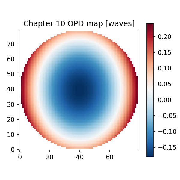
Source and validation note
The OPD discussion is intentionally convention-aware. OPD is meaningful only after the reference wavefront or reference geometry is defined. The toy OPD map in this chapter validates the representation and phase conversion; it is not a substitute for production ray aiming, exit-pupil analysis, reference-sphere fitting, or Zernike reporting.
Chapter 11: Pupil Function: Writing the Wavefront as Complex Numbers
At the end of the previous chapter, OPD gave us a new kind of information.
A spot diagram tells us where rays land. A ray fan tells us how real rays deviate from a reference. OPD tells us something more subtle: for each point in the pupil, how far ahead or behind that part of the wavefront is compared with the ideal reference wavefront.
That is already a big step. But OPD by itself is still not ready to make an image.
To compute a diffraction PSF, the computer needs to know how light from the whole pupil interferes at the image plane. That means it needs two things at each pupil point:
- How much light gets through.
- What phase that light has.
These two pieces are exactly what the pupil function stores.
The pupil function is the moment where wavefront error becomes a complex-valued array. It is the bridge between geometric optical path error and Fourier optics.
This chapter is short in concept but important in the chain:
OPD map
→ pupil amplitude
→ pupil phase
→ complex pupil function
→ PSF
The next chapter will take the Fourier transform of this complex pupil function and turn it into a PSF. Here, we prepare the input carefully.
Do not rush this step. Many wrong PSF and MTF calculations begin with a pupil function that was built with the wrong units, the wrong mask, or the wrong sign convention.
1. The black box we are opening
A diffraction calculation often appears in books as one elegant line:
PSF is related to the Fourier transform of the pupil function.
That statement is true under the usual Fraunhofer approximation, but it hides a practical question:
What exactly is the pupil function in code?
It is not just the aperture shape.
It is not just the OPD map.
It is not just a phase image.
It is a complex-valued function over the pupil:
where:
- is the complex pupil function.
- is the pupil amplitude.
- is the OPD or wavefront error.
- is the wavelength.
- is the imaginary unit.
- are pupil coordinates.
This formula is the whole chapter in one line.
But one line is not enough. We need to know what each part means, how to sample it, and how to write it without lying to ourselves.
2. The aperture mask: where light exists
Start with the simplest part: the aperture.
For an ideal circular pupil, light passes through points inside a circle and is blocked outside it. In normalized pupil coordinates, we can write:
Inside the pupil:
Outside the pupil:
So the simplest aperture mask is:
This mask is not yet the full pupil function. It only says where light is allowed to pass.
In code, this becomes a boolean array:
mask = rho <= 1.0
That one line matters. Without it, your FFT will include light from outside the pupil. The result may still look like a pattern, but it is no longer the PSF of the optical system you intended to model.
This is a useful habit in computational optics:
A wrong array can still produce a beautiful image.
The computer does not know whether your pupil is physical. It only executes the numbers you give it.
3. Pupil amplitude: not always just 1
For a clear, ideal, uniformly illuminated circular aperture, the amplitude is usually written as:
That means:
- amplitude is 1 inside the pupil;
- amplitude is 0 outside the pupil.
This is the simplest case, and it is the right place to begin.
But in real optical systems, amplitude can be more complicated. It may include:
- vignetting;
- central obstruction;
- spider vanes in telescopes;
- transmission variation;
- apodization;
- polarization-dependent effects;
- coating or material transmission differences.
For example, a telescope with a central obstruction has a mask like this:
A system with apodization might have a smooth amplitude such as:
inside the aperture.
For this chapter, we will mostly use the simple circular pupil. But it is important to keep the distinction clear:
mask: where light is allowed
amplitude: how much field amplitude passes through
intensity: amplitude squared
Amplitude is not intensity. If intensity transmission is , then field amplitude is usually proportional to:
That square root is a common source of mistakes. If you put intensity directly into a field amplitude array, your PSF energy will be wrong.
For now, we will keep:
amplitude = mask.astype(float)
That is enough to build the first pupil function.
4. OPD becomes phase
The OPD map tells us how much optical path difference each pupil point has.
If the OPD at one point is , then the corresponding phase is:
This is the key conversion.
The unit rule is simple but strict:
W and λ must use the same length unit.
If is in meters, must be in meters.
If is in micrometers, must be in micrometers.
If is in nanometers and is in meters, the code will still run, but the phase will be wrong by a factor of . There is no warning. There is only a bad result.
Let us make the physical meaning concrete.
Suppose the wavelength is:
If OPD is one full wavelength:
then:
That point has completed one full phase cycle.
If OPD is half a wavelength:
then:
That point is half a cycle out of phase.
This is why a small OPD can matter so much. A few hundred nanometers is tiny mechanically, but optically it can be a large fraction of a visible wavelength.
The pupil function stores this phase as a complex number:
So the full pupil function becomes:
or, substituting phase:
This is the cleanest form to remember.
5. Why complex numbers are not decorative here
It is tempting to think of complex numbers as mathematical decoration. Here they are not decoration. They are how we store phase.
A real-valued OPD map says:
this pupil point is ahead or behind by this much optical path
A complex pupil function says:
this pupil point contributes this amplitude with this phase
When we later compute a PSF, light from different pupil points will interfere. Interference depends on phase.
Two parts of the pupil can have the same amplitude but opposite phase. They may partially cancel. Two parts can have aligned phase. They may reinforce.
That is why a spot diagram cannot fully replace a diffraction calculation. A spot diagram treats rays as landing points. A pupil function prepares the wave nature of light for coherent summation.
Here is the important shift:
Geometric ray tracing asks:
Where does this ray go?
Wave optics asks:
How do all pupil contributions add together as complex fields?
The pupil function is where we prepare the answer to the second question.
6. A minimal pupil grid
Now we write the first version in Python.
We will use normalized pupil coordinates. That means the pupil radius is 1, and the coordinate range is roughly:
x from -1 to 1
y from -1 to 1
This is not yet a physical length in millimeters. It is a normalized coordinate system. That is fine for this chapter because we are focusing on the conversion:
OPD → phase → complex pupil
Here is the grid:
import numpy as np
import matplotlib.pyplot as plt
def make_pupil_grid(n=256):
"""
Create a square sampling grid with normalized pupil coordinates.
Returns
-------
x, y : 2D arrays
Normalized pupil coordinates.
rho : 2D array
Radial pupil coordinate.
theta : 2D array
Angular pupil coordinate.
mask : 2D boolean array
True inside the unit circular pupil.
"""
coord = np.linspace(-1.0, 1.0, n)
x, y = np.meshgrid(coord, coord)
rho = np.sqrt(x**2 + y**2)
theta = np.arctan2(y, x)
mask = rho <= 1.0
return x, y, rho, theta, mask
The output arrays all have shape:
(n, n)
A square grid is convenient for FFTs, even though the physical pupil is circular. The circular aperture is represented by the mask.
This is one of the first small compromises of numerical optics:
The computational array is square.
The optical aperture may not be.
The mask tells the array what is physically real.
That distinction will become very important in the next chapter.
7. A simple OPD map
In a real optical design program, OPD is computed from the optical system. Rays are traced through the surfaces, optical path length is accumulated, and the wavefront is compared with a reference sphere or reference wave.
For learning, we can begin with a synthetic OPD map. This lets us test the pupil function machinery without needing a full lens model in every example.
We will create a simple wavefront with two components:
- Defocus-like variation.
- Astigmatism-like variation.
This is not a full Zernike implementation. It is only a compact way to create a recognizable OPD pattern.
def synthetic_opd(rho, theta, mask, wavelength):
"""
Create a synthetic OPD map in meters.
This is a teaching wavefront, not a full optical design result.
The coefficients are fractions of wavelength.
"""
opd = np.zeros_like(rho)
# Coefficients in meters
defocus = 0.50 * wavelength
astigmatism = 0.25 * wavelength
# Simple wavefront terms
opd += defocus * (2.0 * rho**2 - 1.0)
opd += astigmatism * rho**2 * np.cos(2.0 * theta)
# Outside the pupil, OPD is not physically meaningful.
# We keep it at zero numerically, but the mask will block it.
opd[~mask] = 0.0
return opd
The important part is not the exact polynomial. The important part is that opd is an array with the same shape as the pupil grid.
Each sampled pupil point now has a wavefront error.
grid point → OPD value → phase value → complex pupil value
That is the conversion we want to make explicit.
8. Building the complex pupil function
Now we can write the function that does the main job of the chapter.
def pupil_function_from_opd(opd, mask, wavelength, amplitude=None):
"""
Convert an OPD map into a complex pupil function.
Parameters
----------
opd : 2D array
Optical path difference, in meters.
mask : 2D boolean array
True inside the aperture.
wavelength : float
Wavelength in meters.
amplitude : 2D array or None
Field amplitude transmission. If None, use a clear aperture.
Returns
-------
pupil : 2D complex array
Complex pupil function.
phase : 2D array
Phase in radians.
"""
if amplitude is None:
amplitude = mask.astype(float)
phase = 2.0 * np.pi * opd / wavelength
pupil = amplitude * np.exp(1j * phase)
# Make sure the field is zero outside the aperture.
pupil[~mask] = 0.0 + 0.0j
return pupil, phase
This function is small, but it is doing a very important conversion.
Let us run it:
wavelength = 550e-9 # 550 nm, in meters
x, y, rho, theta, mask = make_pupil_grid(n=256)
opd = synthetic_opd(rho, theta, mask, wavelength)
pupil, phase = pupil_function_from_opd(
opd=opd,
mask=mask,
wavelength=wavelength
)
At this point:
opdis a real-valued array in meters.phaseis a real-valued array in radians.pupilis a complex-valued array.
You can check:
print(opd.dtype)
print(phase.dtype)
print(pupil.dtype)
The third one should be complex.
Use this as a sanity check. If your pupil function is not complex, then you have not yet stored phase in a form that can interfere.
A very common Python 3 typo looks like this:
print phase.dtype
That line is not valid Python 3. It should be:
print(phase.dtype)
This is a small reminder: in computational optics, many mistakes are not grand theoretical mistakes. Some are simply syntax, shape, unit, or convention mistakes. Catch them early.
9. Visualizing OPD, phase, and amplitude
Before moving to PSF, always look at the pupil data.
A good rule is:
Never Fourier-transform a pupil function you have not inspected.
We can plot three things:
- OPD in waves.
- Wrapped phase.
- Amplitude mask.
OPD in waves is:
This is often easier to interpret than meters.
def show_pupil_maps(opd, phase, pupil, mask, wavelength):
opd_waves = opd / wavelength
wrapped_phase = np.angle(pupil)
opd_plot = np.where(mask, opd_waves, np.nan)
phase_plot = np.where(mask, wrapped_phase, np.nan)
amp_plot = np.abs(pupil)
plt.figure(figsize=(5, 4))
plt.imshow(opd_plot, origin="lower", extent=[-1, 1, -1, 1])
plt.colorbar(label="OPD [waves]")
plt.title("OPD map")
plt.xlabel("Normalized pupil x")
plt.ylabel("Normalized pupil y")
plt.tight_layout()
plt.show()
plt.figure(figsize=(5, 4))
plt.imshow(phase_plot, origin="lower", extent=[-1, 1, -1, 1])
plt.colorbar(label="Wrapped phase [rad]")
plt.title("Pupil phase")
plt.xlabel("Normalized pupil x")
plt.ylabel("Normalized pupil y")
plt.tight_layout()
plt.show()
plt.figure(figsize=(5, 4))
plt.imshow(amp_plot, origin="lower", extent=[-1, 1, -1, 1])
plt.colorbar(label="Field amplitude")
plt.title("Pupil amplitude")
plt.xlabel("Normalized pupil x")
plt.ylabel("Normalized pupil y")
plt.tight_layout()
plt.show()
show_pupil_maps(opd, phase, pupil, mask, wavelength)
There are a few things to notice.
The OPD map may look smooth and continuous.
The phase map may appear to jump suddenly. That does not necessarily mean the wavefront is discontinuous. It may only mean that phase is wrapped between and .
This is a common source of confusion.
The complex exponential does not care whether phase is written as:
or:
Those are the same point on the unit circle.
So when you plot phase using np.angle, you are usually seeing wrapped phase. Wrapped phase is useful, but it can make smooth wavefronts look like they contain sharp jumps.
The OPD map is often better for understanding the physical wavefront. The wrapped phase map is better for checking the complex field that will go into the FFT.
10. Phase wrapping is not automatically an error
Let us pause here because this mistake is very common.
Suppose the OPD gradually increases from 0 to one wavelength across the pupil. The phase increases from:
to:
But np.angle usually displays complex phase in the range:
So when phase passes , the plotted value jumps to .
That jump looks dramatic, but it may only be a display convention.
The complex number itself is continuous around the unit circle:
and:
So the two edges of the displayed jump may represent nearly the same complex value.
This is why you should inspect both:
OPD in waves
wrapped phase
OPD tells you the physical wavefront error.
Wrapped phase tells you the phase as stored in the complex pupil.
They answer related but different questions.
11. A clear circular aperture with no aberration
Before using an aberrated wavefront, it helps to build the perfect case.
If OPD is zero everywhere inside the pupil:
then:
For a clear circular aperture:
So the pupil function is just a flat disk of complex value .
zero_opd = np.zeros_like(rho)
perfect_pupil, perfect_phase = pupil_function_from_opd(
opd=zero_opd,
mask=mask,
wavelength=wavelength
)
print(np.max(np.abs(perfect_pupil)))
print(np.min(np.abs(perfect_pupil[mask])))
Inside the pupil, the amplitude should be 1.
Outside the pupil, the field should be 0.
This perfect pupil is the input that will produce the familiar diffraction-limited Airy pattern in the next chapter.
At this stage, we are not yet calculating the Airy pattern. We are only preparing the field that produces it.
The chain is:
flat circular pupil
→ Fourier transform
→ Airy-like PSF
Aberrations modify the pupil phase. They do not necessarily change the pupil amplitude.
So an aberrated pupil may still have amplitude 1 inside the aperture, but its phase is no longer flat.
That is the central idea:
A clear aberrated system can have uniform amplitude but non-uniform phase.
12. Adding a central obstruction
Now let us modify only the amplitude.
This example is useful because it separates two effects:
- aperture shape affects amplitude;
- OPD affects phase.
A central obstruction can be represented by blocking the middle of the pupil.
def annular_amplitude(rho, inner_radius=0.3):
"""
Field amplitude for an annular pupil.
"""
return ((rho >= inner_radius) & (rho <= 1.0)).astype(float)
amplitude_annular = annular_amplitude(rho, inner_radius=0.3)
annular_pupil, annular_phase = pupil_function_from_opd(
opd=zero_opd,
mask=mask,
wavelength=wavelength,
amplitude=amplitude_annular
)
Here the OPD is still zero. The phase is still flat. But the pupil amplitude has changed.
That means the PSF will change even without aberration.
This is an important lesson:
Not every PSF change comes from wavefront error.
Some PSF changes come from aperture shape and amplitude transmission.
If you model a telescope and forget the central obstruction, your diffraction pattern will be wrong even if your OPD is perfect.
If you model vignetting incorrectly, your PSF and MTF can change because the pupil amplitude changed.
Again, beautiful output is not proof of correct input.
13. What Optiland contributes at this step
Our minimal code has used a synthetic OPD map. That is useful for learning, but it is not how a real lens analysis normally begins.
In a real optical system, the OPD should come from the optical prescription:
surfaces
→ materials
→ wavelengths
→ fields
→ pupil sampling
→ ray tracing
→ reference wavefront
→ OPD map
This is where a tool such as Optiland becomes useful. The educational pattern should be:
Use Optiland or another optical design library to compute OPD from a real system.
Then use the same pupil-function formula to understand what happens next.
The exact API can change across versions, so the safest way to write this in a book project is to lock the library version in the companion code. Conceptually, the workflow looks like this:
# Version-checked workflow.
# Check the installed Optiland version and documentation
# before using exact class and method names.
# 1. Build or load an optical system.
# optic = ...
# 2. Choose field and wavelength.
# field = ...
# wavelength = 550e-9
# 3. Run wavefront / OPD analysis.
# wavefront = ...
# opd = wavefront.opd_map(...)
# 4. Get or define the pupil mask.
# mask = wavefront.pupil_mask(...)
# 5. Convert OPD to a complex pupil function.
# pupil, phase = pupil_function_from_opd(opd, mask, wavelength)
This is not meant to replace Optiland’s internal PSF tools. Instead, it explains the bridge.
If Optiland gives you an OPD map, you now know what the next mathematical step is:
And if Optiland directly gives you a PSF, you now know one of the hidden inputs that PSF calculation depends on.
That is the point of the double-track method in this book.
The library performs the complete engineering workflow. The minimal code lets you see the calculation skeleton.
14. Sign convention: the quiet source of disagreement
There is one detail we should treat carefully: the sign in the exponential.
You may see pupil functions written as:
or:
Both conventions appear in optics and signal processing contexts, often depending on the Fourier transform convention and the definition of OPD.
This is annoying, but it is manageable.
The rule is not “one sign is always correct.” The rule is:
Use a consistent sign convention across OPD, pupil function, Fourier transform, and coordinate definitions.
For intensity PSF alone, changing the sign of a real phase function often produces a related or mirrored result. But when you care about phase-sensitive quantities, asymmetric aberrations, coherent imaging, or comparing against a software package, the convention matters.
For this book’s minimal code, we will use:
If your software package uses the opposite convention, do not panic. Check its documentation, then adapt the sign in your comparison code.
A practical comparison checklist is:
- Use the same wavelength.
- Use the same pupil coordinate orientation.
- Use the same OPD reference.
- Use the same phase sign convention.
- Use the same FFT convention when moving to PSF.
When two programs disagree, the first suspect should not be “the physics is wrong.” The first suspects should be units, signs, sampling, and normalization.
15. Pupil coordinates: physical or normalized?
In this chapter we used normalized coordinates:
with the circular pupil defined by:
This is convenient for teaching.
In a real optical system, pupil coordinates may also be expressed in physical units, such as millimeters. A pupil radius might be:
Then a physical pupil coordinate can be normalized as:
The OPD itself is not automatically normalized. OPD remains a length.
So you might have:
x, y: normalized pupil coordinates
W: meters
λ: meters
phase: radians
That combination is perfectly fine.
The coordinate system describes where you are in the pupil. OPD and wavelength describe how much phase delay exists there.
Keep these roles separate:
pupil coordinate: position
OPD: path difference
wavelength: scale for phase conversion
phase: angle in radians
When this separation is clear, the code becomes much easier to debug.
16. The pupil function is not the PSF
This is worth saying plainly.
The pupil function is not the image of a point source.
The pupil function lives in the pupil plane. It describes the complex field across the aperture.
The PSF lives in the image plane. It describes intensity distribution after diffraction and aberration.
The next chapter will connect them through a Fourier transform, but they are not the same object.
A rough map is:
Pupil plane:
complex field over aperture
Image plane:
intensity distribution around image point
This matters because a phase map can look severe while the resulting PSF may still be compact, or a small-looking pupil obstruction can produce visible diffraction rings.
You cannot always read the final image quality directly from one pupil plot. The pupil function is the input. The PSF is the output after coherent propagation.
That is why we are building the chain carefully instead of jumping straight to the final plot.
17. A complete minimal script
Here is a compact version of the whole chapter’s minimal implementation.
It creates:
- a pupil grid;
- a circular mask;
- a synthetic OPD map;
- a complex pupil function;
- plots for OPD, phase, and amplitude.
import numpy as np
import matplotlib.pyplot as plt
def make_pupil_grid(n=256):
coord = np.linspace(-1.0, 1.0, n)
x, y = np.meshgrid(coord, coord)
rho = np.sqrt(x**2 + y**2)
theta = np.arctan2(y, x)
mask = rho <= 1.0
return x, y, rho, theta, mask
def synthetic_opd(rho, theta, mask, wavelength):
opd = np.zeros_like(rho)
defocus = 0.50 * wavelength
astigmatism = 0.25 * wavelength
opd += defocus * (2.0 * rho**2 - 1.0)
opd += astigmatism * rho**2 * np.cos(2.0 * theta)
opd[~mask] = 0.0
return opd
def pupil_function_from_opd(opd, mask, wavelength, amplitude=None):
if amplitude is None:
amplitude = mask.astype(float)
phase = 2.0 * np.pi * opd / wavelength
pupil = amplitude * np.exp(1j * phase)
pupil[~mask] = 0.0 + 0.0j
return pupil, phase
def plot_map(data, title, colorbar_label):
plt.figure(figsize=(5, 4))
plt.imshow(data, origin="lower", extent=[-1, 1, -1, 1])
plt.colorbar(label=colorbar_label)
plt.title(title)
plt.xlabel("Normalized pupil x")
plt.ylabel("Normalized pupil y")
plt.tight_layout()
plt.show()
wavelength = 550e-9
x, y, rho, theta, mask = make_pupil_grid(n=256)
opd = synthetic_opd(rho, theta, mask, wavelength)
pupil, phase = pupil_function_from_opd(
opd=opd,
mask=mask,
wavelength=wavelength
)
opd_waves = np.where(mask, opd / wavelength, np.nan)
wrapped_phase = np.where(mask, np.angle(pupil), np.nan)
amplitude = np.abs(pupil)
plot_map(opd_waves, "OPD map", "OPD [waves]")
plot_map(wrapped_phase, "Wrapped pupil phase", "Phase [rad]")
plot_map(amplitude, "Pupil amplitude", "Field amplitude")
This script does not yet calculate the PSF. That is deliberate.
At this point, the correct question is not:
Where is the image?
The correct question is:
Have we correctly built the complex field that will form the image?
Once that answer is yes, the Fourier transform in the next chapter will make sense.
18. Common mistakes
Let us collect the most common errors before moving on.
Mistake 1: Mixing units
This is the most dangerous one.
Wrong:
opd = 200 # nanometers, but not labeled
wavelength = 550e-9 # meters
phase = 2 * np.pi * opd / wavelength
Correct:
opd = 200e-9
wavelength = 550e-9
phase = 2 * np.pi * opd / wavelength
Always make OPD and wavelength use the same unit.
Mistake 2: Forgetting the aperture mask
If you compute:
pupil = np.exp(1j * phase)
without applying the mask, you have allowed light through the whole square array.
Correct:
pupil = mask.astype(float) * np.exp(1j * phase)
pupil[~mask] = 0.0
The FFT does not know your aperture is supposed to be circular unless you tell it.
Mistake 3: Confusing amplitude and intensity
If a filter transmits 25% of intensity, the field amplitude factor is not 0.25. It is:
Wrong:
amplitude = intensity_transmission
Usually correct:
amplitude = np.sqrt(intensity_transmission)
This matters because PSF intensity is calculated from the squared magnitude of a complex field.
Mistake 4: Thinking wrapped phase jumps are always physical jumps
A sudden jump in np.angle(pupil) may only be phase wrapping.
Check OPD in waves before deciding the wavefront is discontinuous.
Mistake 5: Comparing against software without checking conventions
If your PSF differs from a software package, check:
- wavelength;
- pupil sampling;
- OPD reference;
- phase sign;
- FFT shift;
- normalization;
- coordinate orientation.
Do this before changing the physics.
Mistake 6: Treating the pupil function as a final result
The pupil function is an intermediate representation. It is extremely important, but it is not the PSF and not the MTF.
Its job is to carry amplitude and phase information into the diffraction calculation.
19. What this chapter adds to the full chain
We can now update the book’s main computation chain:
lens prescription
→ surfaces and materials
→ ray tracing
→ optical path length
→ OPD map
→ pupil amplitude
→ pupil phase
→ complex pupil function
This chapter performed one precise conversion:
OPD in length units
→ phase in radians
→ complex field over the aperture
That conversion is small enough to fit in a few lines of code. But conceptually, it is one of the most important steps in the book.
Without it, OPD remains only a wavefront error map.
With it, the wavefront becomes something that can interfere, diffract, and form an image.
That is why the pupil function is the doorway into PSF calculation.
In the next chapter, we will send this complex pupil function through a Fourier transform. The result will no longer live in the pupil plane. It will become the intensity distribution of a point image: the PSF.
And from that PSF, we will finally be close to the MTF curve that started this whole journey.
Chapter summary
The pupil function stores the complex field across the aperture.
It combines:
amplitude
phase
aperture mask
The central formula is:
where OPD must use the same length unit as wavelength .
The aperture mask tells the code where light exists. The amplitude tells how much field passes through. The phase tells how OPD changes the complex field.
A perfect clear circular pupil has flat phase and uniform amplitude. An aberrated pupil may have uniform amplitude but non-uniform phase. An obstructed or apodized pupil may have non-uniform amplitude even with zero OPD.
The main code action in this chapter was:
phase = 2.0 * np.pi * opd / wavelength
pupil = amplitude * np.exp(1j * phase)
pupil[~mask] = 0.0
That is the bridge from OPD to Fourier optics.
Next, we will use this pupil function to compute the PSF.
Generated validation figure
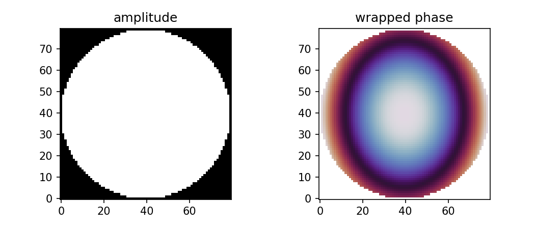
Chapter 12: How PSF Is Computed from a Pupil Function
A point source should be the simplest possible object.
It has no size. It has no texture. It has no edge, no pattern, no detail. In geometric optics, a perfect lens would take all rays from that point and bring them back to one point in the image plane.
But real optical systems do not make mathematical points.
Even a perfect circular aperture spreads a point into a small diffraction pattern. Aberrations spread it further, deform it, shift energy out of the center, or produce asymmetric tails.
That spread-out image of a point is the point spread function, or PSF.
The previous chapter built the object that diffraction calculation needs:
This is the complex pupil function. It stores aperture amplitude and wavefront phase.
Now we let that pupil function form an image.
The short computational chain is:
complex pupil function
→ Fourier transform
→ complex image-plane field
→ squared magnitude
→ PSF
In code, the skeleton is short:
field = np.fft.fftshift(np.fft.fft2(np.fft.ifftshift(pupil)))
psf = np.abs(field) ** 2
psf = psf / np.sum(psf)
Those three lines are the center of this chapter.
But they are not magic. We need to unpack what they mean, what assumptions they use, and what can go wrong.
1. What the PSF represents
The PSF is the intensity distribution produced in the image plane by a point object.
If the optical system were perfect and there were no diffraction, the PSF would be an infinitely small point. But physical light has wavelength, and apertures have finite size. A finite aperture cannot focus light into an infinitely small spot.
For a circular, aberration-free pupil, the ideal diffraction pattern is the familiar Airy pattern:
- a bright central core;
- surrounding rings;
- decreasing intensity away from the center.
This is the diffraction-limited PSF.
When aberrations are present, the pupil phase is no longer flat. The Fourier transform of that distorted complex pupil redistributes energy in the image plane. The PSF changes shape.
So the PSF is not merely a pretty picture. It answers a concrete imaging question:
If the object contains one ideal point, what intensity pattern does the system draw in the image?
Once we know that, we are very close to understanding blur, resolution, and MTF.
2. From pupil plane to image plane
The pupil function lives in the pupil plane. It tells us the complex field across the aperture.
The PSF lives in the image plane. It tells us the intensity around the focused point image.
Under the usual scalar Fraunhofer diffraction approximation, the complex field in the focal region is proportional to the Fourier transform of the pupil function:
The PSF is the squared magnitude of that complex field:
Combining the two:
where:
- is the complex pupil function;
- is the complex image-plane field;
- are image-plane or angular coordinates;
- denotes a Fourier transform.
The proportionality sign matters. A real physical PSF needs correct coordinate scaling and energy normalization. For learning the computational chain, we can first compute a normalized PSF:
That means the PSF is treated as an energy distribution. The total energy is one, and we study where that energy goes.
This normalization is simple and useful:
psf = psf / np.sum(psf)
It does not solve every physical scaling problem, but it makes comparisons between different pupil functions much clearer.
3. Why the Fourier transform appears
The Fourier transform appears because the image-plane field is built by coherent addition of contributions from all pupil points.
Each point in the pupil contributes a small wave. In the far field or focal plane approximation, the phase relationship between those contributions changes with image-plane position. The Fourier transform is the mathematical operation that sums all those complex contributions for each output position.
This is the part that ray diagrams hide.
A ray diagram says:
This part of the pupil sends light in this direction.
A diffraction calculation says:
All pupil points contribute complex amplitudes, and these amplitudes interfere.
The PSF is produced by interference.
That is why the pupil function must be complex. If we only kept OPD as a real-valued map, we would know wavefront error, but we would not yet have the object needed for coherent summation.
The chain now looks like this:
OPD map
→ phase map
→ complex pupil function
→ coherent Fourier summation
→ image-plane intensity
This is the moment where wavefront error becomes visible blur.
4. A perfect circular pupil
Start with the simplest case: a clear circular aperture with no aberration.
Inside the pupil:
So:
Outside the pupil:
This flat circular pupil produces the diffraction-limited Airy pattern.
Let us reuse the pupil grid idea from the previous chapter.
import numpy as np
import matplotlib.pyplot as plt
def make_pupil_grid(n=256):
coord = np.linspace(-1.0, 1.0, n)
x, y = np.meshgrid(coord, coord)
rho = np.sqrt(x**2 + y**2)
theta = np.arctan2(y, x)
mask = rho <= 1.0
return x, y, rho, theta, mask
def pupil_function_from_opd(opd, mask, wavelength, amplitude=None):
if amplitude is None:
amplitude = mask.astype(float)
phase = 2.0 * np.pi * opd / wavelength
pupil = amplitude * np.exp(1j * phase)
pupil[~mask] = 0.0 + 0.0j
return pupil, phase
Now create a perfect pupil:
wavelength = 550e-9 # meters
x, y, rho, theta, mask = make_pupil_grid(n=256)
zero_opd = np.zeros_like(rho)
perfect_pupil, perfect_phase = pupil_function_from_opd(
opd=zero_opd,
mask=mask,
wavelength=wavelength
)
The pupil is complex, but in this perfect case its phase is zero inside the aperture. So the complex value is simply:
inside the circle.
Now we are ready to compute the PSF.
5. Computing a PSF with FFT
A discrete Fourier transform is computed with numpy.fft.fft2.
Because we usually want the central peak in the middle of the displayed image, we use fftshift.
A careful version uses ifftshift before the transform and fftshift after it:
def compute_psf(pupil, normalize=True):
"""
Compute a normalized PSF from a complex pupil function.
Parameters
----------
pupil : 2D complex array
Complex pupil function.
normalize : bool
If True, normalize total PSF energy to 1.
Returns
-------
psf : 2D array
Intensity PSF.
field : 2D complex array
Complex field in the image plane.
"""
field = np.fft.fftshift(
np.fft.fft2(
np.fft.ifftshift(pupil)
)
)
psf = np.abs(field) ** 2
if normalize:
total = np.sum(psf)
if total > 0:
psf = psf / total
return psf, field
Run it:
perfect_psf, perfect_field = compute_psf(perfect_pupil)
This perfect_psf array is the diffraction-limited PSF for our sampled circular pupil.
It is not yet labeled in micrometers or arcseconds. It is a sampled Fourier-plane result. We will return to coordinate scaling later in the chapter.
First, look at the pattern.
6. Displaying the PSF
A PSF usually has a very bright central peak and much weaker surrounding structure. If you display it linearly, the center may dominate so strongly that the rings are hard to see.
So we often display both:
- linear intensity;
- logarithmic intensity.
def show_psf(psf, title="PSF"):
plt.figure(figsize=(5, 4))
plt.imshow(psf, origin="lower")
plt.colorbar(label="Normalized intensity")
plt.title(title + " - linear scale")
plt.xlabel("Image sample x")
plt.ylabel("Image sample y")
plt.tight_layout()
plt.show()
plt.figure(figsize=(5, 4))
plt.imshow(np.log10(psf + 1e-12), origin="lower")
plt.colorbar(label="log10 intensity")
plt.title(title + " - log scale")
plt.xlabel("Image sample x")
plt.ylabel("Image sample y")
plt.tight_layout()
plt.show()
show_psf(perfect_psf, title="Diffraction-limited circular pupil")
The logarithmic plot is not a different PSF. It is the same PSF shown with a display transform.
This distinction matters. A log-scale PSF can make weak rings look visually important. A linear-scale PSF can hide structure that still affects MTF. Good analysis often needs both views.
A sensible habit is:
Use linear scale to judge energy concentration.
Use log scale to inspect weak structure.
The central peak is usually the most important part for sharpness, but the faint surrounding energy tells you where contrast has gone.
7. Zero padding: making the displayed PSF smoother
The FFT output sampling depends on the input array size. If the pupil array is small, the PSF may look blocky or under-sampled.
A common technique is to zero-pad the pupil before the FFT.
Zero padding does not add new optical information. It interpolates the Fourier-domain display more finely.
Here is a padded PSF function:
def pad_array_centered(array, pad_factor=2):
"""
Zero-pad a 2D array around its center.
Parameters
----------
array : 2D array
Input array.
pad_factor : int
Output size will be pad_factor times the input size.
Returns
-------
padded : 2D array
Centered zero-padded array.
"""
if pad_factor == 1:
return array
n, m = array.shape
new_n = n * pad_factor
new_m = m * pad_factor
padded = np.zeros((new_n, new_m), dtype=array.dtype)
start_n = (new_n - n) // 2
start_m = (new_m - m) // 2
padded[start_n:start_n + n, start_m:start_m + m] = array
return padded
def compute_psf(pupil, pad_factor=2, normalize=True):
"""
Compute a PSF from a complex pupil function, with optional zero padding.
"""
padded_pupil = pad_array_centered(pupil, pad_factor=pad_factor)
field = np.fft.fftshift(
np.fft.fft2(
np.fft.ifftshift(padded_pupil)
)
)
psf = np.abs(field) ** 2
if normalize:
total = np.sum(psf)
if total > 0:
psf = psf / total
return psf, field
Now compute a smoother display:
perfect_psf, perfect_field = compute_psf(
perfect_pupil,
pad_factor=4
)
show_psf(perfect_psf, title="Diffraction-limited PSF with zero padding")
Again, zero padding is not magic resolution. It gives us more output samples between the same physical features.
A useful way to say it:
Zero padding makes the plotted PSF smoother.
It does not make the optical system sharper.
That sentence prevents many bad interpretations.
8. Reading the perfect PSF
The perfect circular-pupil PSF has three major features.
First, the central peak is compact and symmetric. This is the Airy core.
Second, rings surround the central peak. These rings are not aberrations. They are diffraction from a finite circular aperture.
Third, the pattern is radially symmetric because the pupil is radially symmetric and the phase is flat.
This is an important baseline.
If the optical system has a circular clear aperture and no aberration, the PSF is not a point. It is already spread out by diffraction.
So when someone says “diffraction-limited,” they do not mean “infinitely sharp.” They mean the system is limited mainly by diffraction rather than aberration.
In practice:
perfect wavefront + finite aperture
→ diffraction-limited PSF
distorted wavefront + finite aperture
→ aberrated PSF
A PSF can only be judged correctly relative to this baseline. The right comparison is not against a mathematical point. The right comparison is against the diffraction-limited PSF for the same aperture and wavelength.
9. Adding aberration
Now let us reuse a synthetic OPD map. We will make a defocus-like and astigmatism-like wavefront, just as in the previous chapter.
def synthetic_opd(rho, theta, mask, wavelength):
"""
Create a synthetic OPD map in meters.
This is a teaching wavefront, not a full optical design result.
"""
opd = np.zeros_like(rho)
defocus = 0.50 * wavelength
astigmatism = 0.25 * wavelength
opd += defocus * (2.0 * rho**2 - 1.0)
opd += astigmatism * rho**2 * np.cos(2.0 * theta)
opd[~mask] = 0.0
return opd
Build the aberrated pupil:
aberrated_opd = synthetic_opd(
rho=rho,
theta=theta,
mask=mask,
wavelength=wavelength
)
aberrated_pupil, aberrated_phase = pupil_function_from_opd(
opd=aberrated_opd,
mask=mask,
wavelength=wavelength
)
aberrated_psf, aberrated_field = compute_psf(
aberrated_pupil,
pad_factor=4
)
Now display it:
show_psf(aberrated_psf, title="Aberrated PSF")
Compared with the perfect PSF, the aberrated PSF should show energy redistributed away from the center. Depending on the aberration, the central peak may broaden, become asymmetric, or develop side structure.
This is the central visual lesson of the chapter:
Aberration is phase error in the pupil.
The PSF shows where that phase error sends the image energy.
A wavefront map may look abstract. The PSF shows its consequence.
10. Comparing perfect and aberrated PSFs
A side-by-side display is useful.
def show_two_psfs(psf_a, psf_b, title_a, title_b, log_scale=False):
if log_scale:
image_a = np.log10(psf_a + 1e-12)
image_b = np.log10(psf_b + 1e-12)
label = "log10 intensity"
else:
image_a = psf_a
image_b = psf_b
label = "Normalized intensity"
vmin = min(np.nanmin(image_a), np.nanmin(image_b))
vmax = max(np.nanmax(image_a), np.nanmax(image_b))
plt.figure(figsize=(10, 4))
plt.subplot(1, 2, 1)
plt.imshow(image_a, origin="lower", vmin=vmin, vmax=vmax)
plt.colorbar(label=label)
plt.title(title_a)
plt.xlabel("Image sample x")
plt.ylabel("Image sample y")
plt.subplot(1, 2, 2)
plt.imshow(image_b, origin="lower", vmin=vmin, vmax=vmax)
plt.colorbar(label=label)
plt.title(title_b)
plt.xlabel("Image sample x")
plt.ylabel("Image sample y")
plt.tight_layout()
plt.show()
show_two_psfs(
perfect_psf,
aberrated_psf,
"Perfect PSF",
"Aberrated PSF",
log_scale=False
)
show_two_psfs(
perfect_psf,
aberrated_psf,
"Perfect PSF",
"Aberrated PSF",
log_scale=True
)
The linear comparison tells us how much energy remains concentrated near the center.
The log comparison shows faint structure.
Both matter. If the central energy drops, fine detail contrast usually suffers. If faint energy spreads far away, the image can gain halos or low-level blur.
This is why PSF is more informative than a single number. It shows the spatial shape of the blur.
MTF, which we will compute in the next chapter, compresses this spatial information into frequency response. That is powerful, but it also hides some visible structure. The PSF lets us see the blur directly.
11. Encircled energy: a simple PSF summary
Before going to MTF, it is useful to introduce one simple PSF-based summary: encircled energy.
Encircled energy asks:
How much of the total PSF energy lies inside a given radius?
This is not the same as MTF, but it is often useful. A sharper PSF concentrates energy into a smaller radius.
Here is a simple implementation in pixel units:
def encircled_energy(psf):
"""
Compute encircled energy as a function of radius in pixel units.
Parameters
----------
psf : 2D array
Normalized PSF.
Returns
-------
radii : 1D array
Radius values in pixels.
energy : 1D array
Encircled energy for each radius.
"""
n, m = psf.shape
cy = (n - 1) / 2.0
cx = (m - 1) / 2.0
yy, xx = np.indices(psf.shape)
r = np.sqrt((xx - cx)**2 + (yy - cy)**2)
r_flat = r.ravel()
psf_flat = psf.ravel()
order = np.argsort(r_flat)
r_sorted = r_flat[order]
psf_sorted = psf_flat[order]
cumulative = np.cumsum(psf_sorted)
return r_sorted, cumulative
Plot perfect versus aberrated:
r_perfect, e_perfect = encircled_energy(perfect_psf)
r_aberr, e_aberr = encircled_energy(aberrated_psf)
plt.figure(figsize=(6, 4))
plt.plot(r_perfect, e_perfect, label="Perfect")
plt.plot(r_aberr, e_aberr, label="Aberrated")
plt.xlabel("Radius [pixels]")
plt.ylabel("Encircled energy")
plt.title("Encircled energy comparison")
plt.legend()
plt.grid(True)
plt.tight_layout()
plt.show()
If the aberrated PSF spreads energy outward, its encircled energy curve rises more slowly.
This gives us a simple way to say:
The aberrated system needs a larger radius to contain the same fraction of point-source energy.
Again, this is not a replacement for MTF. It is another way of looking at image formation.
PSF is spatial. Encircled energy summarizes spatial concentration. MTF will describe spatial frequency response.
They are connected, but they are not identical.
12. Strehl ratio: central peak as a warning light
Another common PSF-based quantity is the Strehl ratio.
In simple computational terms, Strehl ratio compares the peak intensity of an aberrated PSF with the peak intensity of the diffraction-limited PSF, under matching normalization and sampling:
Code:
def strehl_ratio(aberrated_psf, perfect_psf):
return np.max(aberrated_psf) / np.max(perfect_psf)
strehl = strehl_ratio(aberrated_psf, perfect_psf)
print(strehl)
A lower Strehl ratio means the central peak has lost energy relative to the ideal diffraction-limited case.
This is a useful warning light, but it is not a full image-quality description.
Two PSFs can have similar peak values but different shapes. One may have symmetric broadening; another may have a comet-like tail. Their visual effects can differ.
So the rule is:
Strehl ratio summarizes the central peak.
The PSF image shows the whole blur structure.
The PSF still deserves to be looked at.
13. Why spot diagrams and PSFs are different
At this point, it is worth comparing PSF with the spot diagram from earlier chapters.
A spot diagram comes from traced rays. It shows where rays intersect the image plane.
A PSF comes from diffraction calculation. It uses the complex pupil function, including phase, and computes interference.
They may tell similar stories for badly aberrated systems, but they are not the same calculation.
A spot diagram answers:
Where do sampled rays land?
A PSF answers:
What intensity distribution does a point source produce after wave interference?
For large aberrations, the geometric spot can give a useful first impression of blur. But near the diffraction limit, a spot diagram can be misleading. It may show a tight ray bundle and still fail to show diffraction rings. It also does not directly tell us how energy is distributed by interference.
This is one reason optical software provides multiple plots:
- spot diagram;
- ray fan;
- OPD;
- PSF;
- MTF.
They are not redundant. They are different projections of the same optical system.
The full computational route matters:
ray tracing
→ OPD
→ pupil function
→ PSF
The spot diagram branches off from ray intersections. The PSF branches off from wavefront phase.
That difference is the heart of Part Four of this book.
14. The Airy pattern and the diffraction limit
For a perfect circular aperture, the analytic PSF is the Airy pattern. Its intensity profile is commonly written in terms of a Bessel function. We do not need the full analytic derivation here, but we should know the practical meaning.
The first dark ring occurs at an angular radius approximately:
where:
- is angular radius in radians;
- is wavelength;
- is aperture diameter.
At the focal plane, the corresponding radius is approximately:
where is the f-number.
This tells us something physically important:
Longer wavelength gives a larger diffraction spot.
Smaller aperture diameter gives a larger diffraction spot.
Larger f-number gives a larger diffraction spot.
This is why stopping down a lens can improve aberrations but worsen diffraction blur. The PSF is shaped by both aberration and aperture size.
Our FFT computation has reproduced the structure of the Airy pattern from the pupil function. To assign physical units to the output samples, we need aperture size, focal length, wavelength, and sampling relationships. That full scaling is important in engineering use, but the core generation mechanism is already visible:
clear circular pupil
→ Fourier transform
→ Airy-like PSF
That is the computational fact we needed first.
15. Coordinate scaling: what the FFT output means
The FFT returns samples in a frequency-like coordinate. If the pupil coordinate is normalized, the output coordinate is also in a normalized reciprocal coordinate. That is fine for comparing shapes, but physical interpretation needs scaling.
For a physical aperture field sampled over pupil coordinates , the focal-plane coordinates are related to diffraction angles. Roughly:
where are spatial frequency coordinates associated with the pupil-plane sampling.
At the focal plane of a lens with focal length :
The exact implementation depends on how you sampled the physical pupil and how you define the Fourier transform normalization.
For this chapter, the safest practical division is:
First compute the correct normalized PSF shape.
Then attach physical coordinates using known aperture sampling, wavelength, and focal length.
Trying to do both at once often confuses beginners.
Here is a simple coordinate helper for a physical pupil diameter:
def psf_angular_coordinates(n_output, pupil_sample_spacing, wavelength):
"""
Estimate angular coordinates for FFT-based Fraunhofer PSF.
Parameters
----------
n_output : int
Number of samples in the padded pupil / PSF array.
pupil_sample_spacing : float
Physical pupil-plane sample spacing, in meters.
wavelength : float
Wavelength, in meters.
Returns
-------
theta : 1D array
Angular coordinate samples, in radians.
"""
freq = np.fft.fftshift(
np.fft.fftfreq(n_output, d=pupil_sample_spacing)
)
theta = wavelength * freq
return theta
If your original pupil diameter is , and the unpadded pupil grid has samples across the full square coordinate range, a rough sample spacing is:
pupil_sample_spacing = D / n
Then:
D = 5e-3 # 5 mm aperture diameter
n_input = perfect_pupil.shape[0]
pad_factor = 4
n_output = n_input * pad_factor
dx_pupil = D / n_input
theta = psf_angular_coordinates(
n_output=n_output,
pupil_sample_spacing=dx_pupil,
wavelength=wavelength
)
This gives angular samples in radians. If the focal length is known, convert to focal-plane length:
focal_length = 50e-3 # 50 mm
image_coord = focal_length * theta
This coordinate scaling is useful, but it also deserves caution. The more realistic your model becomes, the more carefully you must define:
- pupil diameter;
- entrance pupil versus exit pupil;
- focal length;
- image-space refractive index;
- sampling convention;
- FFT normalization;
- field point;
- wavelength.
For now, remember the main warning:
The PSF array is easy to compute.
The physical coordinate labels require careful bookkeeping.
Chapter 14 will return to sampling and normalization more aggressively.
16. A complete minimal PSF script
Here is a compact script that builds both perfect and aberrated PSFs.
import numpy as np
import matplotlib.pyplot as plt
def make_pupil_grid(n=256):
coord = np.linspace(-1.0, 1.0, n)
x, y = np.meshgrid(coord, coord)
rho = np.sqrt(x**2 + y**2)
theta = np.arctan2(y, x)
mask = rho <= 1.0
return x, y, rho, theta, mask
def synthetic_opd(rho, theta, mask, wavelength):
opd = np.zeros_like(rho)
defocus = 0.50 * wavelength
astigmatism = 0.25 * wavelength
opd += defocus * (2.0 * rho**2 - 1.0)
opd += astigmatism * rho**2 * np.cos(2.0 * theta)
opd[~mask] = 0.0
return opd
def pupil_function_from_opd(opd, mask, wavelength, amplitude=None):
if amplitude is None:
amplitude = mask.astype(float)
phase = 2.0 * np.pi * opd / wavelength
pupil = amplitude * np.exp(1j * phase)
pupil[~mask] = 0.0 + 0.0j
return pupil, phase
def pad_array_centered(array, pad_factor=2):
if pad_factor == 1:
return array
n, m = array.shape
new_n = n * pad_factor
new_m = m * pad_factor
padded = np.zeros((new_n, new_m), dtype=array.dtype)
start_n = (new_n - n) // 2
start_m = (new_m - m) // 2
padded[start_n:start_n + n, start_m:start_m + m] = array
return padded
def compute_psf(pupil, pad_factor=4, normalize=True):
padded_pupil = pad_array_centered(pupil, pad_factor=pad_factor)
field = np.fft.fftshift(
np.fft.fft2(
np.fft.ifftshift(padded_pupil)
)
)
psf = np.abs(field) ** 2
if normalize:
total = np.sum(psf)
if total > 0:
psf = psf / total
return psf, field
def show_two_psfs(psf_a, psf_b, title_a, title_b, log_scale=False):
if log_scale:
image_a = np.log10(psf_a + 1e-12)
image_b = np.log10(psf_b + 1e-12)
label = "log10 intensity"
else:
image_a = psf_a
image_b = psf_b
label = "Normalized intensity"
vmin = min(np.nanmin(image_a), np.nanmin(image_b))
vmax = max(np.nanmax(image_a), np.nanmax(image_b))
plt.figure(figsize=(10, 4))
plt.subplot(1, 2, 1)
plt.imshow(image_a, origin="lower", vmin=vmin, vmax=vmax)
plt.colorbar(label=label)
plt.title(title_a)
plt.xlabel("Image sample x")
plt.ylabel("Image sample y")
plt.subplot(1, 2, 2)
plt.imshow(image_b, origin="lower", vmin=vmin, vmax=vmax)
plt.colorbar(label=label)
plt.title(title_b)
plt.xlabel("Image sample x")
plt.ylabel("Image sample y")
plt.tight_layout()
plt.show()
wavelength = 550e-9
x, y, rho, theta, mask = make_pupil_grid(n=256)
zero_opd = np.zeros_like(rho)
perfect_pupil, _ = pupil_function_from_opd(
opd=zero_opd,
mask=mask,
wavelength=wavelength
)
aberrated_opd = synthetic_opd(
rho=rho,
theta=theta,
mask=mask,
wavelength=wavelength
)
aberrated_pupil, _ = pupil_function_from_opd(
opd=aberrated_opd,
mask=mask,
wavelength=wavelength
)
perfect_psf, _ = compute_psf(perfect_pupil, pad_factor=4)
aberrated_psf, _ = compute_psf(aberrated_pupil, pad_factor=4)
show_two_psfs(
perfect_psf,
aberrated_psf,
"Perfect PSF",
"Aberrated PSF",
log_scale=False
)
show_two_psfs(
perfect_psf,
aberrated_psf,
"Perfect PSF",
"Aberrated PSF",
log_scale=True
)
strehl = np.max(aberrated_psf) / np.max(perfect_psf)
print("Approximate Strehl ratio:", strehl)
This script is still a teaching model. It does not replace a full optical design package. But it exposes the calculation skeleton clearly:
make pupil
→ add phase from OPD
→ FFT
→ square magnitude
→ normalize
→ compare
That is exactly the hidden step we wanted to open.
17. Connecting this to Optiland
In a real Optiland workflow, you would usually not hand-create the OPD map from a synthetic polynomial. You would define or load an optical system, select a field point and wavelength, and then ask the analysis tools for wavefront or PSF results.
Conceptually, the flow is:
Optiland optical system
→ ray tracing and wavefront analysis
→ pupil function or equivalent internal representation
→ PSF analysis
A validation-style comparison workflow looks like this:
# Version-checked workflow outline.
# Check your installed Optiland version for exact API names.
# 1. Build or load an optical system.
# optic = ...
# 2. Select field and wavelength.
# field = ...
# wavelength = ...
# 3. Compute wavefront / OPD using Optiland analysis tools.
# wavefront = ...
# opd = wavefront.opd_map(...)
# 4. Build a pupil function from that OPD.
# pupil, phase = pupil_function_from_opd(opd, mask, wavelength)
# 5. Compute a teaching PSF using NumPy.
# psf_numpy, field_numpy = compute_psf(pupil, pad_factor=4)
# 6. Compute PSF using Optiland's own PSF analysis.
# psf_optiland = ...
# 7. Compare shape, normalization, sampling, and coordinate scaling.
Twenty lines of NumPy do not replace a mature optical design tool. They make the hidden calculation inspectable.
When Optiland gives you a PSF, you should now be able to ask:
- What pupil was sampled?
- What wavelength was used?
- What field point was used?
- What OPD or phase was included?
- What aperture mask was applied?
- What FFT sampling and normalization were used?
- Is the plot linear or logarithmic?
- Are the coordinates image-plane, angular, or normalized?
These questions are more valuable than memorizing a button sequence.
A tool can produce the PSF. Understanding means knowing what had to happen for that PSF to exist.
18. Common mistakes in PSF calculation
Mistake 1: Taking the Fourier transform of OPD directly
OPD is not the pupil function.
Wrong:
psf = np.abs(np.fft.fft2(opd)) ** 2
Correct:
phase = 2.0 * np.pi * opd / wavelength
pupil = amplitude * np.exp(1j * phase)
psf = np.abs(np.fft.fft2(pupil)) ** 2
The FFT operates on the complex field, not on OPD as a height map.
Mistake 2: Forgetting to square the magnitude
The Fourier transform gives a complex field. The PSF is intensity.
Wrong:
psf = np.fft.fft2(pupil)
Correct:
field = np.fft.fft2(pupil)
psf = np.abs(field) ** 2
Intensity is squared magnitude.
Mistake 3: Comparing unnormalized PSFs
If two PSFs have different total sums, peak comparisons can be misleading.
Better:
psf = psf / np.sum(psf)
Then you can compare energy distribution more fairly.
Mistake 4: Believing zero padding increases resolution
Zero padding makes the PSF display smoother. It does not improve the physical optical resolution.
Mistake 5: Ignoring display scale
A linear plot and a log plot can make the same PSF feel very different.
Always check which scale is being used before interpreting rings, halos, or faint tails.
Mistake 6: Forgetting that PSF depends on wavelength and field
A PSF is not a universal property of a lens.
It depends on:
- wavelength;
- field point;
- focus position;
- aperture;
- pupil sampling;
- polarization assumptions if included;
- aberration state.
A single PSF plot is one slice through a larger optical behavior.
19. What this chapter adds to the full chain
We can now extend the computation chain:
lens prescription
→ surfaces and materials
→ ray tracing
→ optical path length
→ OPD map
→ pupil amplitude and phase
→ complex pupil function
→ Fourier transform
→ PSF
The new step is:
with normalization applied for practical comparison.
That is a major milestone.
We have moved from geometric rays to a wave-optical image of a point. We have also seen why a point never remains a point in a real optical system.
A clear circular pupil produces a diffraction-limited Airy-like pattern. An aberrated pupil changes phase across the aperture and redistributes energy in the PSF. An obstructed or apodized pupil changes amplitude and also changes the PSF.
The PSF is where aperture, diffraction, and aberration meet in image space.
The next chapter will take one more step. Instead of asking how one point is blurred, we will ask how different spatial frequencies are transmitted.
That takes us from PSF to OTF, and then to MTF.
The MTF curve that looked like a software output in Chapter 1 is now almost within reach.
Chapter summary
The PSF is the image-plane intensity distribution produced by an ideal point source.
Under the usual scalar Fraunhofer diffraction approximation, the complex image-plane field is proportional to the Fourier transform of the complex pupil function:
The PSF is the squared magnitude of that field:
In minimal NumPy code:
field = np.fft.fftshift(np.fft.fft2(np.fft.ifftshift(pupil)))
psf = np.abs(field) ** 2
psf = psf / np.sum(psf)
A perfect clear circular pupil produces a diffraction-limited Airy-like PSF. An aberrated pupil redistributes energy away from the ideal central peak. A changed aperture amplitude also changes the PSF, even if the wavefront phase is flat.
The PSF should be inspected carefully, often in both linear and logarithmic display. Zero padding can make the displayed PSF smoother, but it does not improve the actual optical resolution.
Most importantly, the FFT must be applied to the complex pupil function, not directly to the OPD map.
The computation chain now reaches:
OPD
→ pupil function
→ PSF
Next, we will ask how this PSF acts on image detail at different spatial frequencies. That question leads to the OTF and MTF.
Generated validation figure
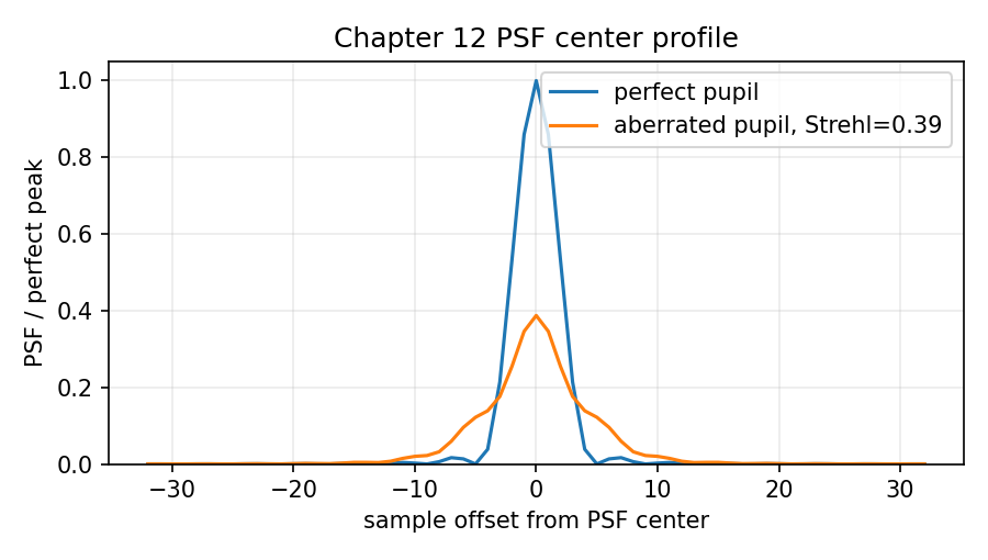
Source and validation note
The PSF computation in this chapter uses the scalar Fourier-optics model appropriate for teaching the pupil-to-image calculation. It deliberately omits vector diffraction, polarization effects, partial coherence, detector sampling, and detailed physical units. Those omissions are boundaries of the chapter, not claims that those effects are unimportant.
Chapter 13: OTF and MTF: Turning a PSF into a Frequency Response
We began this book with a curve.
An MTF curve appears in optical design software as if it were a finished verdict: sharp here, weak there, better in one field, worse in another. It looks clean. It looks authoritative. It is easy to read just enough of it to become dangerous.
But an MTF curve is not born as a curve.
It is the end of a calculation chain.
By now, that chain is no longer hidden:
lens prescription
→ ray tracing
→ optical path length
→ OPD
→ pupil function
→ PSF
→ OTF
→ MTF
In Chapter 12, we computed the PSF from the complex pupil function. The PSF told us how one ideal point spreads out in the image plane.
Now we ask a different question:
If the object contains patterns of different spatial frequencies,
how strongly does the optical system transfer each one?
That question leads to the optical transfer function, or OTF.
The MTF, or modulation transfer function, is the magnitude of the OTF.
In minimal form:
Those two lines are simple. Their meaning is not small.
This chapter is where the PSF stops being only an image of a point and becomes a frequency response.
1. Why MTF exists at all
The PSF answers:
What does the system do to one point?
MTF answers:
What does the system do to contrast at different detail sizes?
An object can be thought of as containing many spatial frequencies.
Large, slow changes are low spatial frequencies. Fine details are high spatial frequencies.
For example:
- a broad gray patch is low frequency;
- a thick black-white stripe pattern is lower frequency;
- a very fine stripe pattern is higher frequency;
- tiny texture, hair, fabric weave, or fine printed text contains high frequencies.
An optical system does not transmit all these frequencies equally.
Low-frequency contrast may survive well. High-frequency contrast may be weakened. At some point, fine detail may no longer be transferred with useful contrast.
That is what the MTF curve shows.
A typical MTF curve begins near 1 at zero frequency and drops as frequency increases.
This does not mean every system drops smoothly in every direction. Real systems can have structure, directional differences, field dependence, wavelength dependence, and sampling issues. But the first mental model is:
MTF tells us how contrast transfer changes with spatial frequency.
That sentence is useful. It is also incomplete. The rest of the chapter makes it computable.
2. PSF as an impulse response
To understand why the Fourier transform of the PSF gives the OTF, we need one idea from imaging theory.
For an incoherent, shift-invariant imaging system, the image can be modeled as the object blurred by the PSF.
In compact notation:
where means convolution.
This says:
The final image is made by replacing each object point
with a copy of the PSF and adding all those copies together.
That is a powerful idea.
If the PSF is narrow, points remain concentrated, and the image looks sharp.
If the PSF is broad, each object point spreads more widely, and the image loses fine detail.
The convolution theorem then tells us:
The Fourier transform of the PSF is the system’s transfer function:
So the OTF tells us how each spatial frequency component of the object is changed by the optical system.
This is why PSF and OTF are two views of the same imaging behavior:
PSF: spatial-domain blur
OTF: frequency-domain transfer
They are not separate measurements floating in space. They are a Fourier pair.
3. OTF is complex; MTF is its magnitude
The OTF is generally complex:
It has:
- magnitude;
- phase.
The magnitude is the MTF:
The phase is often called the phase transfer function, or PTF:
Many optical design discussions focus on MTF because contrast transfer is extremely useful. But MTF throws away the phase part of the OTF.
That is not a small detail.
The MTF tells you how much contrast remains at each spatial frequency. It does not fully tell you where structures move, whether phase reversals occur, or how asymmetric blur affects image appearance.
This is one of the central judgments of this book:
MTF is important, but it is not the whole image-quality story.
That is not an argument against MTF. It is an argument against treating one curve as if it contained every optical truth.
PSF, OTF phase, field dependence, wavelength dependence, distortion, sensor sampling, and image processing can all matter.
For now, we will compute the OTF and MTF directly from the PSF. Then we will learn how to read the result without worshiping it.
4. Normalization: why MTF starts at 1
The zero-frequency component represents the average brightness transfer. For a normalized PSF whose total energy is one:
the OTF value at zero frequency should also be one:
So the MTF at zero frequency is:
In numerical code, small scaling differences can appear depending on FFT conventions. The safest practical approach is to normalize the OTF by its zero-frequency value:
Then:
This makes the MTF begin at one.
In code, after shifting the FFT output so zero frequency is at the center:
center = (otf.shape[0] // 2, otf.shape[1] // 2)
otf = otf / otf[center]
mtf = np.abs(otf)
This small normalization step prevents a lot of confusion.
If your MTF does not start at 1, do not immediately change the optical model. First check normalization.
5. Computing OTF and MTF from PSF
Let us build directly on the code from the previous chapter.
We will keep the same conceptual flow:
pupil function
→ PSF
→ OTF
→ MTF
Here is the minimal OTF/MTF function:
import numpy as np
def compute_otf_mtf(psf):
"""
Compute the optical transfer function and modulation transfer function
from a normalized or unnormalized PSF.
Parameters
----------
psf : 2D array
Point spread function.
Returns
-------
otf : 2D complex array
Normalized optical transfer function.
mtf : 2D array
Modulation transfer function.
"""
otf = np.fft.fftshift(
np.fft.fft2(
np.fft.ifftshift(psf)
)
)
center = (otf.shape[0] // 2, otf.shape[1] // 2)
if np.abs(otf[center]) > 0:
otf = otf / otf[center]
mtf = np.abs(otf)
return otf, mtf
The structure mirrors the PSF calculation, but the object is different.
In Chapter 12:
FFT of complex pupil → complex image field
squared magnitude → PSF
Here:
FFT of PSF → OTF
magnitude → MTF
Do not mix those two steps.
A common wrong calculation is to take the FFT of the pupil and call its magnitude the MTF. That skips the PSF-to-OTF relationship and confuses coherent field propagation with incoherent image transfer.
The correct chain in this chapter is:
PSF first.
Then OTF.
Then MTF.
6. Reusing the PSF code
For completeness, here is the small working set of functions we need.
This is not a full optical design program. It is the exposed calculation skeleton.
import numpy as np
import matplotlib.pyplot as plt
def make_pupil_grid(n=256):
coord = np.linspace(-1.0, 1.0, n)
x, y = np.meshgrid(coord, coord)
rho = np.sqrt(x**2 + y**2)
theta = np.arctan2(y, x)
mask = rho <= 1.0
return x, y, rho, theta, mask
def pupil_function_from_opd(opd, mask, wavelength, amplitude=None):
if amplitude is None:
amplitude = mask.astype(float)
phase = 2.0 * np.pi * opd / wavelength
pupil = amplitude * np.exp(1j * phase)
pupil[~mask] = 0.0 + 0.0j
return pupil, phase
def pad_array_centered(array, pad_factor=2):
if pad_factor == 1:
return array
n, m = array.shape
new_n = n * pad_factor
new_m = m * pad_factor
padded = np.zeros((new_n, new_m), dtype=array.dtype)
start_n = (new_n - n) // 2
start_m = (new_m - m) // 2
padded[start_n:start_n + n, start_m:start_m + m] = array
return padded
def compute_psf(pupil, pad_factor=4, normalize=True):
padded_pupil = pad_array_centered(pupil, pad_factor=pad_factor)
field = np.fft.fftshift(
np.fft.fft2(
np.fft.ifftshift(padded_pupil)
)
)
psf = np.abs(field) ** 2
if normalize:
total = np.sum(psf)
if total > 0:
psf = psf / total
return psf, field
def compute_otf_mtf(psf):
otf = np.fft.fftshift(
np.fft.fft2(
np.fft.ifftshift(psf)
)
)
center = (otf.shape[0] // 2, otf.shape[1] // 2)
if np.abs(otf[center]) > 0:
otf = otf / otf[center]
mtf = np.abs(otf)
return otf, mtf
Now we can make a perfect circular pupil and compute its PSF and MTF.
wavelength = 550e-9
x, y, rho, theta, mask = make_pupil_grid(n=256)
zero_opd = np.zeros_like(rho)
perfect_pupil, _ = pupil_function_from_opd(
opd=zero_opd,
mask=mask,
wavelength=wavelength
)
perfect_psf, _ = compute_psf(
perfect_pupil,
pad_factor=4
)
perfect_otf, perfect_mtf = compute_otf_mtf(perfect_psf)
At this point, perfect_mtf is a 2D array.
That matters. MTF is not born as one curve. It is first a two-dimensional frequency response:
The familiar curve is usually a slice through this 2D function.
That slice can be horizontal, vertical, sagittal, tangential, radial, or averaged, depending on context.
The curve is not the whole object. It is a chosen view.
7. Displaying the 2D MTF
Let us look at the 2D MTF first.
def show_mtf_2d(mtf, title="MTF"):
plt.figure(figsize=(5, 4))
plt.imshow(mtf, origin="lower", vmin=0, vmax=1)
plt.colorbar(label="MTF")
plt.title(title)
plt.xlabel("Frequency sample x")
plt.ylabel("Frequency sample y")
plt.tight_layout()
plt.show()
show_mtf_2d(perfect_mtf, title="Diffraction-limited 2D MTF")
For a perfect circular pupil, the 2D MTF should be radially symmetric. It is highest at the center, then decreases toward the cutoff.
This is the frequency-domain counterpart of the diffraction-limited PSF.
The PSF showed the Airy-like blur pattern in space.
The MTF shows how that blur reduces contrast at different spatial frequencies.
One is not more real than the other. They are two representations of the same imaging behavior.
Narrow PSF
→ stronger high-frequency transfer
Broad PSF
→ weaker high-frequency transfer
The relationship is not merely visual. It comes from the Fourier transform.
8. Extracting simple MTF curves
Most optical design software does not show only a 2D MTF map. It often shows one-dimensional curves.
For an on-axis, rotationally symmetric system, a horizontal or vertical slice through the MTF center may be enough for a simple demonstration.
Let us extract central slices.
def central_mtf_slices(mtf):
"""
Extract horizontal and vertical MTF slices through the center.
Returns
-------
freq_index : 1D array
Sample index relative to zero frequency.
horizontal : 1D array
MTF along the horizontal frequency axis.
vertical : 1D array
MTF along the vertical frequency axis.
"""
n, m = mtf.shape
cy = n // 2
cx = m // 2
horizontal = mtf[cy, :]
vertical = mtf[:, cx]
freq_index = np.arange(m) - cx
return freq_index, horizontal, vertical
Now plot only the positive-frequency half:
def plot_mtf_slices(mtf, title="MTF slices"):
freq_index, horizontal, vertical = central_mtf_slices(mtf)
center = len(freq_index) // 2
freq_positive = freq_index[center:]
horizontal_positive = horizontal[center:]
vertical_positive = vertical[center:]
plt.figure(figsize=(6, 4))
plt.plot(freq_positive, horizontal_positive, label="Horizontal slice")
plt.plot(freq_positive, vertical_positive, "--", label="Vertical slice")
plt.xlabel("Frequency sample index")
plt.ylabel("MTF")
plt.ylim(0, 1.05)
plt.title(title)
plt.grid(True)
plt.legend()
plt.tight_layout()
plt.show()
plot_mtf_slices(perfect_mtf, title="Diffraction-limited MTF slices")
For the ideal circular pupil, the two curves should be nearly identical. Small numerical differences can come from sampling.
This is our first MTF curve.
It is still in sample-index units, not cycles per millimeter. That is acceptable for understanding the chain. Physical frequency units will require coordinate scaling, and Chapter 14 will spend more time on that.
For now, the important point is:
The curve came from a slice through a 2D MTF,
which came from the Fourier transform of the PSF,
which came from the Fourier transform of the pupil function.
That is the black box opened.
9. Adding aberration and watching MTF fall
Now let us create an aberrated pupil and compare MTF curves.
We use a teaching OPD map again:
def synthetic_opd(rho, theta, mask, wavelength):
"""
Create a synthetic OPD map in meters.
This is a teaching wavefront, not a full optical design result.
"""
opd = np.zeros_like(rho)
defocus = 0.50 * wavelength
astigmatism = 0.25 * wavelength
opd += defocus * (2.0 * rho**2 - 1.0)
opd += astigmatism * rho**2 * np.cos(2.0 * theta)
opd[~mask] = 0.0
return opd
Compute the aberrated PSF and MTF:
aberrated_opd = synthetic_opd(
rho=rho,
theta=theta,
mask=mask,
wavelength=wavelength
)
aberrated_pupil, _ = pupil_function_from_opd(
opd=aberrated_opd,
mask=mask,
wavelength=wavelength
)
aberrated_psf, _ = compute_psf(
aberrated_pupil,
pad_factor=4
)
aberrated_otf, aberrated_mtf = compute_otf_mtf(aberrated_psf)
Now compare central slices:
def plot_mtf_comparison(mtf_a, mtf_b, label_a, label_b, title="MTF comparison"):
freq_index, h_a, v_a = central_mtf_slices(mtf_a)
_, h_b, v_b = central_mtf_slices(mtf_b)
center = len(freq_index) // 2
freq_positive = freq_index[center:]
plt.figure(figsize=(7, 4))
plt.plot(freq_positive, h_a[center:], label=f"{label_a} horizontal")
plt.plot(freq_positive, v_a[center:], "--", label=f"{label_a} vertical")
plt.plot(freq_positive, h_b[center:], label=f"{label_b} horizontal")
plt.plot(freq_positive, v_b[center:], "--", label=f"{label_b} vertical")
plt.xlabel("Frequency sample index")
plt.ylabel("MTF")
plt.ylim(0, 1.05)
plt.title(title)
plt.grid(True)
plt.legend()
plt.tight_layout()
plt.show()
plot_mtf_comparison(
perfect_mtf,
aberrated_mtf,
label_a="Perfect",
label_b="Aberrated",
title="Perfect vs aberrated MTF"
)
The aberrated MTF should fall below the perfect MTF, especially at higher spatial frequencies.
This is not an arbitrary penalty. It comes from energy spreading in the PSF.
A broader or more structured PSF reduces the system’s ability to preserve contrast in fine details.
The chain is:
pupil phase error
→ changed PSF
→ changed OTF
→ lower or direction-dependent MTF
This is the computational story behind a curve that otherwise looks like a software report.
10. Direction matters: sagittal and tangential MTF
Optical design software often plots sagittal and tangential MTF curves.
These names can feel mysterious at first, but the idea is geometric.
For an off-axis field point, there is a plane containing:
- the optical axis;
- the chief ray;
- the field point.
This is the tangential or meridional direction.
The direction perpendicular to it is the sagittal direction.
In a perfectly on-axis rotationally symmetric case, sagittal and tangential behavior is the same. Off-axis, they can differ significantly.
That difference is not cosmetic. Astigmatism, coma, and field-dependent aberrations often affect different directions differently.
In our simplified centered array, we can imitate the idea by treating one central slice as tangential and the perpendicular slice as sagittal.
This is only a teaching simplification.
def sagittal_tangential_slices_simple(mtf):
"""
Simplified sagittal/tangential slices for a centered MTF array.
For a real off-axis field, sagittal and tangential directions should be
defined relative to the field point and optical axis. Here we use
vertical and horizontal central slices as a teaching proxy.
"""
n, m = mtf.shape
cy = n // 2
cx = m // 2
tangential = mtf[cy, :] # horizontal proxy
sagittal = mtf[:, cx] # vertical proxy
freq_index = np.arange(m) - cx
return freq_index, sagittal, tangential
Now plot them:
def plot_sagittal_tangential_simple(mtf, title="Sagittal and tangential MTF"):
freq_index, sagittal, tangential = sagittal_tangential_slices_simple(mtf)
center = len(freq_index) // 2
freq_positive = freq_index[center:]
plt.figure(figsize=(6, 4))
plt.plot(freq_positive, sagittal[center:], label="Sagittal proxy")
plt.plot(freq_positive, tangential[center:], "--", label="Tangential proxy")
plt.xlabel("Frequency sample index")
plt.ylabel("MTF")
plt.ylim(0, 1.05)
plt.title(title)
plt.grid(True)
plt.legend()
plt.tight_layout()
plt.show()
plot_sagittal_tangential_simple(
aberrated_mtf,
title="Simplified sagittal/tangential MTF"
)
In a real lens analysis, you should not casually rename horizontal and vertical slices as sagittal and tangential without knowing the field geometry.
The real definitions depend on the field point.
A safer way to say this is:
Sagittal and tangential MTF are directional slices through the 2D frequency response,
defined relative to the field geometry.
Software hides that geometry for convenience. When learning the computation, we should keep it visible.
11. Frequency units: sample index is not enough
Our plots currently use frequency sample index. This is good enough to verify the computational chain, but it is not enough for engineering interpretation.
Real MTF curves are often plotted against spatial frequency in:
cycles per millimeter
or equivalently:
line pairs per millimeter
A line pair means one bright line plus one dark line, so line pairs per millimeter and cycles per millimeter are often used in the same practical sense.
To label the frequency axis physically, we need the image-plane sample spacing of the PSF.
If the PSF sample spacing is:
then the frequency samples are:
In NumPy:
freq = np.fft.fftshift(np.fft.fftfreq(n, d=dx_image))
where dx_image is in millimeters if you want frequency in cycles per millimeter.
Here is a helper:
def mtf_frequency_axis(n, dx_image):
"""
Create a shifted frequency axis for an MTF array.
Parameters
----------
n : int
Number of samples.
dx_image : float
Image-plane sample spacing.
Returns
-------
freq : 1D array
Spatial frequency samples in cycles per unit of dx_image.
"""
return np.fft.fftshift(np.fft.fftfreq(n, d=dx_image))
If dx_image is in millimeters, frequency is cycles/mm.
Then a positive-frequency MTF plot can use physical units:
def plot_mtf_with_frequency_axis(mtf, dx_image, title="MTF"):
n, m = mtf.shape
cy = n // 2
cx = m // 2
freq = mtf_frequency_axis(m, dx_image)
mtf_slice = mtf[cy, :]
plt.figure(figsize=(6, 4))
plt.plot(freq[cx:], mtf_slice[cx:])
plt.xlabel("Spatial frequency [cycles per unit]")
plt.ylabel("MTF")
plt.ylim(0, 1.05)
plt.title(title)
plt.grid(True)
plt.tight_layout()
plt.show()
This function is structurally correct, but it needs a real dx_image.
And that is where many mistakes enter.
The PSF sample spacing depends on:
- pupil sampling;
- wavelength;
- focal length or image-space scaling;
- zero padding;
- FFT convention.
We introduced a simple angular-coordinate helper in Chapter 12. Chapter 14 will return to this carefully because frequency-axis mistakes are one of the fastest ways to create a convincing but wrong MTF plot.
For now, keep the warning in mind:
Computing the MTF array is easy.
Labeling the frequency axis correctly requires careful sampling bookkeeping.
12. Diffraction-limited cutoff frequency
There is one physical frequency scale worth introducing now.
For an incoherent diffraction-limited circular aperture in air, the cutoff spatial frequency in image space is often written as:
where:
- is the cutoff frequency;
- is wavelength;
- is the f-number.
If wavelength is in millimeters, then is in cycles per millimeter.
The same idea can also be written using numerical aperture:
These formulas are useful because they give the approximate upper frequency where the diffraction-limited incoherent MTF reaches zero.
For example, if:
and:
then:
This does not mean every real lens at f/5.6 delivers excellent contrast near 325 cycles/mm. It means the diffraction-limited cutoff scale is around that value.
Aberrations, defocus, manufacturing errors, sensor sampling, and image processing all affect what is actually useful.
A careful wording is:
The diffraction cutoff gives a physical ceiling.
The actual MTF curve tells us how much contrast remains below that ceiling.
This is a good example of how MTF should be read: not as a mystical score, but as a frequency-by-frequency contrast transfer.
13. Why MTF can go down without the PSF looking terrible
Sometimes a PSF plot does not look dramatically bad, but the MTF curve has clearly dropped.
This is not a contradiction.
The PSF is a spatial image. Our eyes tend to focus on the central core and visible tails. Small redistributions of energy can still affect high-frequency contrast.
MTF is sensitive to how the PSF interacts with sinusoidal patterns of different frequencies.
A small widening of the PSF can reduce high-frequency MTF even when the PSF still looks “pretty sharp” on a display.
This is one reason MTF became such a useful engineering metric.
It can reveal contrast loss in a way that is hard to judge from a PSF image alone.
But the opposite problem also exists. An MTF curve can hide the spatial character of blur. Two systems may have similar MTF at selected frequencies but different PSF shapes. One might produce symmetric blur; another might produce directional tails or halos.
So we should read PSF and MTF together:
PSF shows where point energy goes.
MTF shows how contrast survives by spatial frequency.
Neither view makes the other obsolete.
14. Phase in OTF: what MTF hides
Because MTF is the magnitude of the OTF, it discards OTF phase.
Let us compute and display the OTF phase:
def show_otf_phase(otf, title="OTF phase"):
phase = np.angle(otf)
plt.figure(figsize=(5, 4))
plt.imshow(phase, origin="lower", cmap="twilight")
plt.colorbar(label="Phase [rad]")
plt.title(title)
plt.xlabel("Frequency sample x")
plt.ylabel("Frequency sample y")
plt.tight_layout()
plt.show()
If your Matplotlib installation does not support the "twilight" colormap, use the default colormap:
def show_otf_phase_default(otf, title="OTF phase"):
phase = np.angle(otf)
plt.figure(figsize=(5, 4))
plt.imshow(phase, origin="lower")
plt.colorbar(label="Phase [rad]")
plt.title(title)
plt.xlabel("Frequency sample x")
plt.ylabel("Frequency sample y")
plt.tight_layout()
plt.show()
For symmetric, centered PSFs, OTF phase may be simple. For shifted or asymmetric PSFs, phase can carry important information.
Here is a small demonstration.
If we shift a PSF, its MTF magnitude may remain the same, while the OTF phase changes.
shifted_psf = np.roll(perfect_psf, shift=10, axis=1)
shifted_otf, shifted_mtf = compute_otf_mtf(shifted_psf)
plot_mtf_comparison(
perfect_mtf,
shifted_mtf,
label_a="Original",
label_b="Shifted",
title="MTF before and after PSF shift"
)
The MTF curves may look almost identical. But the image position changed.
That shift is carried in phase, not magnitude.
This is a clean example of the limit of MTF:
MTF can say contrast is preserved.
It may not tell you that the image has shifted.
In many lens-quality contexts, MTF is still very valuable. But if you need full image formation, registration, phase behavior, or asymmetric effects, OTF phase and PSF shape cannot be ignored.
15. MTF and contrast
Why does MTF correspond to contrast?
Imagine an object with sinusoidal intensity variation:
where:
- is the average intensity;
- is modulation or contrast;
- is spatial frequency.
After passing through an imaging system, the same frequency may come out with reduced modulation:
The MTF at that frequency is:
This is the contrast-transfer meaning of MTF.
If MTF is 1, contrast at that frequency is preserved.
If MTF is 0.5, the modulation is cut in half.
If MTF is near 0, that frequency is barely transferred.
This is why MTF is easier to connect to image detail than many raw optical quantities.
Spot size tells us something. OPD tells us something. PSF tells us something. But MTF directly asks:
How much contrast remains at this detail size?
That is why it became a standard image-quality metric.
Still, remember the boundary:
MTF describes contrast transfer for spatial frequencies.
It does not describe every perceptual or geometric property of an image.
That distinction keeps the metric useful without making it magical.
16. A complete minimal PSF-to-MTF script
Here is a compact script that runs the whole route for a perfect and aberrated pupil.
import numpy as np
import matplotlib.pyplot as plt
def make_pupil_grid(n=256):
coord = np.linspace(-1.0, 1.0, n)
x, y = np.meshgrid(coord, coord)
rho = np.sqrt(x**2 + y**2)
theta = np.arctan2(y, x)
mask = rho <= 1.0
return x, y, rho, theta, mask
def pupil_function_from_opd(opd, mask, wavelength, amplitude=None):
if amplitude is None:
amplitude = mask.astype(float)
phase = 2.0 * np.pi * opd / wavelength
pupil = amplitude * np.exp(1j * phase)
pupil[~mask] = 0.0 + 0.0j
return pupil, phase
def synthetic_opd(rho, theta, mask, wavelength):
opd = np.zeros_like(rho)
defocus = 0.50 * wavelength
astigmatism = 0.25 * wavelength
opd += defocus * (2.0 * rho**2 - 1.0)
opd += astigmatism * rho**2 * np.cos(2.0 * theta)
opd[~mask] = 0.0
return opd
def pad_array_centered(array, pad_factor=4):
if pad_factor == 1:
return array
n, m = array.shape
new_n = n * pad_factor
new_m = m * pad_factor
padded = np.zeros((new_n, new_m), dtype=array.dtype)
start_n = (new_n - n) // 2
start_m = (new_m - m) // 2
padded[start_n:start_n + n, start_m:start_m + m] = array
return padded
def compute_psf(pupil, pad_factor=4, normalize=True):
padded_pupil = pad_array_centered(pupil, pad_factor=pad_factor)
field = np.fft.fftshift(
np.fft.fft2(
np.fft.ifftshift(padded_pupil)
)
)
psf = np.abs(field) ** 2
if normalize:
total = np.sum(psf)
if total > 0:
psf = psf / total
return psf, field
def compute_otf_mtf(psf):
otf = np.fft.fftshift(
np.fft.fft2(
np.fft.ifftshift(psf)
)
)
center = (otf.shape[0] // 2, otf.shape[1] // 2)
if np.abs(otf[center]) > 0:
otf = otf / otf[center]
mtf = np.abs(otf)
return otf, mtf
def central_mtf_slices(mtf):
n, m = mtf.shape
cy = n // 2
cx = m // 2
horizontal = mtf[cy, :]
vertical = mtf[:, cx]
freq_index = np.arange(m) - cx
return freq_index, horizontal, vertical
def plot_mtf_comparison(mtf_a, mtf_b, label_a, label_b):
freq_index, h_a, v_a = central_mtf_slices(mtf_a)
_, h_b, v_b = central_mtf_slices(mtf_b)
center = len(freq_index) // 2
freq_positive = freq_index[center:]
plt.figure(figsize=(7, 4))
plt.plot(freq_positive, h_a[center:], label=f"{label_a} horizontal")
plt.plot(freq_positive, v_a[center:], "--", label=f"{label_a} vertical")
plt.plot(freq_positive, h_b[center:], label=f"{label_b} horizontal")
plt.plot(freq_positive, v_b[center:], "--", label=f"{label_b} vertical")
plt.xlabel("Frequency sample index")
plt.ylabel("MTF")
plt.ylim(0, 1.05)
plt.title("MTF comparison")
plt.grid(True)
plt.legend()
plt.tight_layout()
plt.show()
wavelength = 550e-9
x, y, rho, theta, mask = make_pupil_grid(n=256)
zero_opd = np.zeros_like(rho)
perfect_pupil, _ = pupil_function_from_opd(
opd=zero_opd,
mask=mask,
wavelength=wavelength
)
aberrated_opd = synthetic_opd(
rho=rho,
theta=theta,
mask=mask,
wavelength=wavelength
)
aberrated_pupil, _ = pupil_function_from_opd(
opd=aberrated_opd,
mask=mask,
wavelength=wavelength
)
perfect_psf, _ = compute_psf(perfect_pupil, pad_factor=4)
aberrated_psf, _ = compute_psf(aberrated_pupil, pad_factor=4)
perfect_otf, perfect_mtf = compute_otf_mtf(perfect_psf)
aberrated_otf, aberrated_mtf = compute_otf_mtf(aberrated_psf)
plot_mtf_comparison(
perfect_mtf,
aberrated_mtf,
label_a="Perfect",
label_b="Aberrated"
)
This script should now feel less mysterious than the code preview from Chapter 1.
At the beginning of the book, these lines looked like a shortcut:
otf = np.fft.fftshift(np.fft.fft2(psf))
mtf = np.abs(otf)
Now they have a place in the chain.
They are not arbitrary Fourier transforms. They are computing the frequency response of an incoherent imaging system from its point spread function.
That is the difference between using code and understanding code.
17. Optiland comparison workflow
In a real Optiland workflow, MTF should usually be computed by the library’s own analysis tools when you are doing real design work.
The educational value of our NumPy version is different. It lets us check what the tool must be doing conceptually.
A version-checked workflow outline looks like this:
# Version-checked workflow outline.
# Check your installed Optiland version for exact API names.
# 1. Build or load an optical system.
# optic = ...
# 2. Select field, wavelength, aperture, and focus settings.
# field = ...
# wavelength = ...
# 3. Use Optiland's PSF analysis.
# psf_result = ...
# 4. Use Optiland's MTF analysis.
# mtf_result = ...
# 5. Reconstruct a teaching MTF from a PSF if the sampled PSF is available.
# psf_array = ...
# otf_numpy, mtf_numpy = compute_otf_mtf(psf_array)
# 6. Compare:
# - MTF normalization
# - frequency axis
# - sagittal/tangential definitions
# - wavelength and field settings
# - sampling and padding
The comparison is not just about matching plots. It is about asking the right questions:
- Which field point is this MTF for?
- Which wavelength or wavelength weighting is used?
- Is the plotted curve sagittal, tangential, radial, or averaged?
- Is the frequency axis in cycles/mm, cycles/degree, or normalized units?
- Is the PSF diffraction-based or geometric?
- Is the MTF polychromatic or monochromatic?
- Is the image plane refocused?
- What normalization is being used?
This is where the educational value of an open tool becomes clear.
You do not merely press a button. You can inspect the inputs, reproduce simplified pieces, and understand why the result changes.
That does not make the tool unnecessary. It makes the tool less mysterious.
18. Reading an MTF curve carefully
Once you know how the MTF is computed, you can read the curve with better questions.
The low-frequency region
Low frequencies correspond to broad contrast.
If low-frequency MTF is poor, the image may look generally flat or washed out. In a reasonable optical system, low-frequency MTF is often high unless there are severe aberrations, scatter, defocus, or other contrast-reducing effects.
The middle-frequency region
Middle frequencies often correspond to visually important detail.
For camera lenses, this region can strongly affect perceived sharpness. A lens that preserves moderate spatial frequencies well may look crisp even if very high-frequency response is not perfect.
The high-frequency region
High frequencies correspond to fine detail.
High-frequency MTF is sensitive to diffraction, aberration, focus, sampling, and manufacturing. It often drops first.
But high-frequency MTF should not be read alone. A system can have respectable high-frequency response but poor behavior in other ways, such as field curvature, distortion, flare, or directional blur.
The cutoff
The cutoff is the frequency beyond which contrast transfer is essentially zero.
For diffraction-limited incoherent imaging, this is tied to wavelength and numerical aperture. In real imaging systems, useful contrast may become too low before the theoretical cutoff.
A careful reader asks not only:
Where does the curve end?
but also:
How much contrast remains at the frequencies that matter for this application?
That application-dependent question is often more useful.
19. Why MTF is powerful but not万能
MTF became a standard metric because it compresses an enormous amount of imaging behavior into a readable curve.
That is its strength.
It is also its danger.
A single MTF curve may not tell you:
- whether blur is symmetric or asymmetric;
- whether the PSF has long tails;
- whether there is image shift;
- whether phase behavior matters;
- how distortion affects geometry;
- how color channels differ;
- how performance changes across the field;
- how sensor sampling interacts with optical blur;
- how image processing changes final contrast.
Even several MTF curves do not fully replace looking at the PSF, spot diagram, wavefront, field curvature, distortion, and system prescription.
So a better habit is:
Use MTF as a frequency-domain summary,
not as a complete description of the optical system.
This is the measured version of the sharp claim from the beginning of the book:
Being able to read an MTF curve is not the same as understanding where it came from.
Now we can say exactly where it came from.
It came from the PSF.
The PSF came from the complex pupil function.
The pupil function came from amplitude and OPD.
The OPD came from optical path differences computed through the optical system.
That chain is the real subject of this book.
20. Common mistakes in OTF and MTF calculation
Mistake 1: Taking the MTF directly from the pupil
Wrong:
mtf = np.abs(np.fft.fft2(pupil))
This is not the incoherent MTF.
The pupil transform gives the complex image-plane field. You still need the PSF:
field = np.fft.fft2(pupil)
psf = np.abs(field) ** 2
otf = np.fft.fft2(psf)
mtf = np.abs(otf)
The sequence matters.
Mistake 2: Forgetting OTF normalization
If the MTF does not start at 1, check normalization before interpreting the result.
otf = otf / otf[center]
mtf = np.abs(otf)
Mistake 3: Confusing frequency index with physical frequency
An array index is not cycles/mm.
To get physical frequency, you need the image-plane sample spacing.
freq = np.fft.fftshift(np.fft.fftfreq(n, d=dx_image))
The hard part is knowing dx_image correctly.
Mistake 4: Calling horizontal and vertical slices sagittal and tangential without field geometry
For a real off-axis field, sagittal and tangential directions are defined relative to the optical axis and field point.
Horizontal and vertical slices are only a teaching proxy unless the coordinate system is known.
Mistake 5: Ignoring wavelength and field point
MTF changes with wavelength and field position.
A single curve is not “the MTF of the lens” in all conditions. It is the MTF for a specific configuration.
Mistake 6: Treating MTF as a final truth
MTF is powerful. It is not complete.
Use it with PSF, wavefront, spot diagrams, field plots, and knowledge of the imaging task.
21. What this chapter adds to the full chain
We can now write the complete path from wavefront to MTF:
OPD map
→ pupil phase
→ complex pupil function
→ PSF
→ OTF
→ MTF
The new step is:
and:
In code:
otf = np.fft.fftshift(np.fft.fft2(np.fft.ifftshift(psf)))
otf = otf / otf[center]
mtf = np.abs(otf)
That is the curve behind the button.
Not the whole story, but the essential computational skeleton.
We have now reached the destination that Chapter 1 pointed toward. The rest of the book will make this result safer, more practical, and more connected to real optical design.
Chapter 14 will slow down and do something very necessary: it will look at the ways this calculation can go wrong.
Because at this point, we know enough to make impressive mistakes.
Sampling, FFT shifts, frequency axes, normalization, padding, and units can all produce MTF plots that look plausible but mean the wrong thing.
So before we move on to optimization, we need a rescue chapter.
Chapter summary
The PSF describes spatial blur. The OTF describes frequency response. The MTF is the magnitude of the OTF.
For incoherent, shift-invariant imaging:
In code:
otf = np.fft.fftshift(np.fft.fft2(np.fft.ifftshift(psf)))
otf = otf / otf[center]
mtf = np.abs(otf)
The MTF begins at 1 when properly normalized. It usually drops as spatial frequency increases, showing how contrast transfer weakens for finer detail.
A 2D MTF can be sliced into curves. Sagittal and tangential curves are directional slices defined relative to field geometry; horizontal and vertical slices are only a simplified proxy unless the coordinate system is known.
MTF is powerful because it summarizes contrast transfer by spatial frequency. It is limited because it discards OTF phase and compresses spatial blur behavior into selected curves.
The most important result of this chapter is not just the formula. It is the chain:
PSF
→ OTF
→ MTF
Now an MTF curve is no longer a mysterious output. It is a computed consequence of the PSF, which is itself a computed consequence of the pupil function and wavefront error.
Generated validation figure
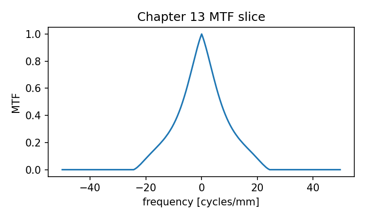
Source and validation note
The OTF/MTF formulas here assume incoherent, shift-invariant imaging and a properly normalized PSF. Real optical-design software may compute diffraction MTF, geometric MTF, polychromatic MTF, field-dependent curves, or direction-specific sagittal/tangential curves under additional conventions. The chapter keeps the core Fourier relationship visible before adding those production details.
Chapter 14: Sampling, Normalization, and the Small Mistakes That Break PSF and MTF
By this point, we have enough code to make convincing plots.
That is good news.
It is also dangerous.
A PSF plot can look smooth and scientific even when the sampling is wrong. An MTF curve can start at 1, fall gracefully, and still have the wrong frequency axis. A Fourier transform can be mathematically valid while representing the wrong physical aperture. A shifted array can produce a result that looks almost right but is centered in the wrong place.
This chapter is a rescue chapter. It adds no new optical concept; it makes the previous three chapters safer.
We have already built this chain:
OPD
→ pupil function
→ PSF
→ OTF
→ MTF
Now we slow down and ask:
When does this chain produce a physically meaningful result?
The answer depends on details that feel small until they break everything:
- FFT shift;
- array centering;
- aperture mask;
- zero padding;
- pupil sampling;
- image-plane sampling;
- frequency-axis units;
- PSF normalization;
- OTF normalization;
- wavelength units;
- focal length units;
- sagittal and tangential directions.
These are not decorative implementation details. They decide what the plot means.
Here is the sharp but useful rule for this chapter:
A correct formula does not save an incorrectly sampled array.
Let us go through the common traps one by one.
1. The problem: beautiful wrong plots
The Fourier transform is extremely obedient.
It does not ask whether your wavelength is in meters or nanometers. It does not know whether your pupil diameter is 5 mm or 5 meters. It does not know whether your zero frequency belongs in the center of the array. It does not know whether your PSF is normalized.
It just transforms the numbers.
That is why FFT-based optics can fail quietly.
A wrong ray-surface intersection often produces an obvious error: rays fly away, intersections disappear, or the code crashes.
A wrong MTF computation may produce a perfectly smooth curve.
This is more dangerous because it looks respectable.
The practical lesson is:
In FFT optics, the first debugging question is not:
“Does the plot look optical?”
It is:
“What are the units, sampling intervals, normalization, and coordinate conventions?”
This chapter gives you a checklist for answering that question.
2. Three arrays, three coordinate systems
The pupil, PSF, and MTF arrays do not live in the same coordinate system.
This is the first source of confusion.
Pupil array
The pupil array describes field across the aperture.
Its coordinates may be:
normalized pupil coordinates
or physical coordinates such as:
meters or millimeters across the pupil
The pupil function is:
where are pupil-plane coordinates.
PSF array
The PSF array describes image-plane intensity.
Its coordinates may be:
angular coordinates
or:
focal-plane length coordinates
The PSF is:
where are image-plane coordinates.
MTF array
The MTF array describes spatial frequency response.
Its coordinates are frequency coordinates:
cycles per millimeter
or:
cycles per radian
or sometimes normalized frequency.
The MTF is:
where are spatial frequencies.
So the chain is not just:
array → array → array
It is:
pupil-plane field
→ image-plane intensity
→ image-plane spatial-frequency response
That distinction saves a lot of debugging time.
3. The DFT sampling relationship
The discrete Fourier transform connects sampling intervals.
If you sample a function with spacing:
and use samples, the corresponding frequency samples are spaced by:
The shifted frequency coordinate is:
for an even-length array after fftshift.
In NumPy, this is:
freq = np.fft.fftshift(np.fft.fftfreq(N, d=dx))
That one line is the safest way to build a frequency axis.
The important parts are:
Nis the number of samples in the transformed array;dxis the sample spacing in the input domain;- the output unit is cycles per unit of
dx.
So if:
dx = 0.01 # millimeters
then:
freq is in cycles per millimeter
If:
dx = 10e-6 # meters
then:
freq is in cycles per meter
The FFT does not attach units. You attach units by using the right dx.
This is the most important sampling idea in the chapter.
4. Pupil sampling to PSF sampling
When we compute a PSF from a pupil function, we are taking a Fourier transform of the pupil field.
For Fraunhofer diffraction, pupil spatial frequency maps to diffraction angle.
A useful practical relationship is:
where:
- is image angle in radians;
- is wavelength;
- is spatial frequency associated with pupil-plane sampling.
If the pupil sample spacing is , and the padded pupil array has samples, then the angular sample spacing is approximately:
At a focal length , focal-plane sample spacing is:
So:
This formula is worth reading slowly.
It says the PSF sample spacing depends on:
- focal length;
- wavelength;
- padded FFT size;
- physical pupil sample spacing.
Zero padding changes , so it changes the displayed PSF sample spacing. It gives more samples in the PSF display.
It does not change the physical aperture.
Here is a helper function:
import numpy as np
def psf_sample_spacing_from_pupil(
wavelength,
focal_length,
pupil_sample_spacing,
n_fft
):
"""
Estimate focal-plane PSF sample spacing for Fraunhofer propagation.
Parameters
----------
wavelength : float
Wavelength in meters.
focal_length : float
Focal length in meters.
pupil_sample_spacing : float
Physical spacing between pupil samples, in meters.
n_fft : int
FFT array size after padding.
Returns
-------
dx_image : float
Approximate image-plane sample spacing, in meters.
"""
dtheta = wavelength / (n_fft * pupil_sample_spacing)
dx_image = focal_length * dtheta
return dx_image
If you want the result in millimeters:
dx_image_mm = dx_image * 1e3
This is the bridge from the pupil array to physical PSF coordinates.
5. Example: a physically labeled PSF
Let us create a simple physical setup.
Suppose:
wavelength = 550 nm
focal length = 50 mm
pupil diameter = 10 mm
The f-number is:
Now build the pupil.
import numpy as np
import matplotlib.pyplot as plt
def make_pupil_grid(n=256):
coord = np.linspace(-1.0, 1.0, n, endpoint=False)
x, y = np.meshgrid(coord, coord)
rho = np.sqrt(x**2 + y**2)
theta = np.arctan2(y, x)
mask = rho <= 1.0
return x, y, rho, theta, mask
def pupil_function_from_opd(opd, mask, wavelength, amplitude=None):
if amplitude is None:
amplitude = mask.astype(float)
phase = 2.0 * np.pi * opd / wavelength
pupil = amplitude * np.exp(1j * phase)
pupil[~mask] = 0.0 + 0.0j
return pupil, phase
def pad_array_centered(array, pad_factor=4):
if pad_factor == 1:
return array
n, m = array.shape
new_n = n * pad_factor
new_m = m * pad_factor
padded = np.zeros((new_n, new_m), dtype=array.dtype)
start_n = (new_n - n) // 2
start_m = (new_m - m) // 2
padded[start_n:start_n + n, start_m:start_m + m] = array
return padded
def compute_psf(pupil, pad_factor=4, normalize=True):
padded_pupil = pad_array_centered(pupil, pad_factor=pad_factor)
field = np.fft.fftshift(
np.fft.fft2(
np.fft.ifftshift(padded_pupil)
)
)
psf = np.abs(field) ** 2
if normalize:
total = np.sum(psf)
if total > 0:
psf = psf / total
return psf, field
Now define the physical parameters:
wavelength = 550e-9 # 550 nm
focal_length = 50e-3 # 50 mm
pupil_diameter = 10e-3 # 10 mm
n_pupil = 256
pad_factor = 4
n_fft = n_pupil * pad_factor
x, y, rho, theta, mask = make_pupil_grid(n=n_pupil)
zero_opd = np.zeros_like(rho)
pupil, _ = pupil_function_from_opd(
opd=zero_opd,
mask=mask,
wavelength=wavelength
)
psf, _ = compute_psf(
pupil,
pad_factor=pad_factor
)
The normalized coordinate grid runs from to , representing the full pupil diameter. So a rough pupil sample spacing is:
In code:
pupil_sample_spacing = pupil_diameter / n_pupil
dx_image = psf_sample_spacing_from_pupil(
wavelength=wavelength,
focal_length=focal_length,
pupil_sample_spacing=pupil_sample_spacing,
n_fft=n_fft
)
dx_image_mm = dx_image * 1e3
print("Image-plane sample spacing [mm]:", dx_image_mm)
print("Image-plane sample spacing [um]:", dx_image * 1e6)
Now we can label the PSF axis.
def image_coordinate_axis(n, dx):
"""
Create centered image-plane coordinate axis.
"""
center = n // 2
index = np.arange(n) - center
return index * dx
coord_image_m = image_coordinate_axis(psf.shape[0], dx_image)
coord_image_um = coord_image_m * 1e6
extent_um = [
coord_image_um[0],
coord_image_um[-1],
coord_image_um[0],
coord_image_um[-1],
]
plt.figure(figsize=(5, 4))
plt.imshow(psf, origin="lower", extent=extent_um)
plt.colorbar(label="Normalized intensity")
plt.xlabel("Image x [um]")
plt.ylabel("Image y [um]")
plt.title("Diffraction-limited PSF with physical axis")
plt.tight_layout()
plt.show()
Now the PSF plot is not just an array image. Its axis has a physical interpretation.
This is a big improvement.
But it also creates responsibility. If the pupil diameter, focal length, wavelength, or padding size is wrong, the axis label is wrong.
6. Checking the Airy radius
A good sanity check is the Airy first dark ring.
For a circular aperture, the first dark ring radius in the focal plane is approximately:
where is the f-number.
With:
λ = 550 nm
N = 5
we get:
Code:
f_number = focal_length / pupil_diameter
airy_radius = 1.22 * wavelength * f_number
print("F-number:", f_number)
print("Airy first dark radius [um]:", airy_radius * 1e6)
This gives us a rough check on the PSF axis.
The first dark ring in the plotted PSF should be near that radius.
It may not match perfectly because of sampling, finite array effects, display interpolation, and how we locate the minimum. But if the ring appears at 3 meters or 0.003 nanometers, something is wrong.
This kind of sanity check is not optional in computational optics.
A good habit is:
After computing a diffraction-limited PSF,
check whether the Airy scale is physically plausible.
This one check catches many unit mistakes.
7. Wrong sampling example: the same PSF with the wrong pupil diameter
Let us intentionally make a mistake.
Suppose the actual pupil diameter is 10 mm, but we accidentally label it as 1 mm.
The computed PSF array does not change. Why? Because the array values came from the normalized pupil mask.
But the physical axis changes dramatically.
wrong_pupil_diameter = 1e-3 # wrong: 1 mm instead of 10 mm
wrong_pupil_sample_spacing = wrong_pupil_diameter / n_pupil
wrong_dx_image = psf_sample_spacing_from_pupil(
wavelength=wavelength,
focal_length=focal_length,
pupil_sample_spacing=wrong_pupil_sample_spacing,
n_fft=n_fft
)
print("Correct dx [um]:", dx_image * 1e6)
print("Wrong dx [um]:", wrong_dx_image * 1e6)
Because the pupil sample spacing became ten times smaller, the image-plane sample spacing becomes ten times larger.
The PSF image still looks like an Airy pattern. But its physical size is mislabeled.
This is the quiet failure mode.
The numerical array is not enough. The coordinate model matters.
The wrong plot may look optical. It may even look beautiful. But it describes a different physical system.
8. From PSF sampling to MTF frequency axis
Now we move one step forward.
The MTF is computed from the PSF. Its frequency axis is determined by the PSF sample spacing.
If the PSF sample spacing is , the MTF frequency samples are:
In NumPy:
freq = np.fft.fftshift(np.fft.fftfreq(N, d=dx_image))
If dx_image is in meters, freq is in cycles per meter.
For cycles per millimeter:
freq_cyc_per_mm = freq / 1000.0
because one meter contains 1000 millimeters, and cycles/m divided by 1000 gives cycles/mm.
Here is a clean MTF computation with axis generation:
def compute_otf_mtf(psf):
otf = np.fft.fftshift(
np.fft.fft2(
np.fft.ifftshift(psf)
)
)
center = (otf.shape[0] // 2, otf.shape[1] // 2)
if np.abs(otf[center]) > 0:
otf = otf / otf[center]
mtf = np.abs(otf)
return otf, mtf
def mtf_frequency_axis(n, dx_image):
"""
Frequency axis for MTF.
Parameters
----------
n : int
Number of PSF / MTF samples.
dx_image : float
PSF sample spacing in meters.
Returns
-------
freq_cyc_per_mm : 1D array
Spatial frequency in cycles/mm.
"""
freq_cyc_per_m = np.fft.fftshift(
np.fft.fftfreq(n, d=dx_image)
)
freq_cyc_per_mm = freq_cyc_per_m / 1000.0
return freq_cyc_per_mm
Now compute and plot:
otf, mtf = compute_otf_mtf(psf)
freq = mtf_frequency_axis(
n=mtf.shape[0],
dx_image=dx_image
)
center = mtf.shape[0] // 2
mtf_slice = mtf[center, :]
plt.figure(figsize=(6, 4))
plt.plot(freq[center:], mtf_slice[center:])
plt.xlabel("Spatial frequency [cycles/mm]")
plt.ylabel("MTF")
plt.ylim(0, 1.05)
plt.title("Diffraction-limited MTF")
plt.grid(True)
plt.tight_layout()
plt.show()
Now the x-axis has a physical meaning.
9. Checking the diffraction cutoff
For incoherent diffraction-limited imaging with a circular aperture, the cutoff frequency is approximately:
where:
- is in cycles per length;
- uses the same length unit;
- is the f-number.
If is in millimeters, is cycles/mm.
wavelength_mm = wavelength * 1e3
cutoff_cyc_per_mm = 1.0 / (wavelength_mm * f_number)
print("Diffraction cutoff [cycles/mm]:", cutoff_cyc_per_mm)
For 550 nm and f/5, the cutoff is approximately:
The MTF should approach zero around that frequency.
Again, it will not be perfect in a small teaching script. But it should be in the right neighborhood.
If your plotted MTF goes to zero at 3.64 cycles/mm or 3,640,000 cycles/mm, suspect a unit error.
The cutoff gives a strong sanity check:
Airy radius checks the PSF axis.
Diffraction cutoff checks the MTF axis.
These two checks should become automatic.
10. Wrong MTF axis example
Let us intentionally make the MTF axis wrong by using the wrong PSF sample spacing.
The MTF values are the same, but the frequency labels change.
wrong_freq = mtf_frequency_axis(
n=mtf.shape[0],
dx_image=wrong_dx_image
)
plt.figure(figsize=(7, 4))
plt.plot(freq[center:], mtf_slice[center:], label="Correct axis")
plt.plot(wrong_freq[center:], mtf_slice[center:], "--", label="Wrong axis")
plt.xlabel("Spatial frequency [cycles/mm]")
plt.ylabel("MTF")
plt.ylim(0, 1.05)
plt.title("Same MTF values, different frequency labels")
plt.grid(True)
plt.legend()
plt.tight_layout()
plt.show()
This is the exact kind of error that can survive visual inspection.
The curve shape is identical. Only the x-axis changes.
But for engineering interpretation, that is not a small problem. It changes the answer to questions like:
What is the MTF at 50 cycles/mm?
What is the cutoff frequency?
How does this compare with a sensor pixel pitch?
A mislabeled frequency axis can turn a weak system into a strong one, or a strong one into a weak one.
The curve shape alone is not enough.
11. FFT shift: where is the center?
FFT shift errors are another classic trap.
NumPy’s FFT functions use an array convention where zero frequency is at the beginning of the array before shifting.
For display and optical interpretation, we often want zero frequency or the PSF peak at the center.
So we use:
np.fft.fftshift(...)
and sometimes:
np.fft.ifftshift(...)
The common pattern for PSF from pupil is:
field = np.fft.fftshift(
np.fft.fft2(
np.fft.ifftshift(pupil)
)
)
The common pattern for OTF from PSF is:
otf = np.fft.fftshift(
np.fft.fft2(
np.fft.ifftshift(psf)
)
)
Keep centered arrays centered through the transform.
There are several valid conventions, but mixing conventions is dangerous.
A practical test:
peak_index = np.unravel_index(np.argmax(psf), psf.shape)
print("PSF peak index:", peak_index)
print("Expected center:", (psf.shape[0] // 2, psf.shape[1] // 2))
For an on-axis perfect pupil, the PSF peak should be at or very near the center.
If it appears in a corner, your shift convention is wrong for your display.
For the MTF:
otf_center = (otf.shape[0] // 2, otf.shape[1] // 2)
print("OTF center value:", otf[otf_center])
print("MTF center value:", mtf[otf_center])
The MTF center should be close to 1 after normalization.
These checks are simple. Use them.
12. Odd and even array sizes
Even-sized and odd-sized arrays have slightly different center behavior.
For an even array with , the center index after fftshift is:
N // 2
For an odd array with , it is also:
N // 2
but the symmetry around the center is slightly different.
This does not mean odd sizes are forbidden. It means you should be consistent and test where the peak and zero frequency appear.
For teaching code, powers of two or even sizes are convenient:
256, 512, 1024
They are not required by modern FFT libraries, but they make examples clean.
When debugging, avoid changing too many things at once. Do not simultaneously change:
- array size;
- padding factor;
- aperture diameter;
- wavelength;
- FFT shift convention.
Change one thing and observe what happens.
That is slow, but it works.
13. Zero padding: interpolation, not extra physics
Zero padding is useful, but it is often misunderstood.
When you zero-pad the pupil before computing the PSF, you increase the number of samples in the Fourier-domain output.
The displayed PSF becomes smoother.
But the physical aperture has not changed. The optical resolution has not improved.
The correct statement is:
Zero padding interpolates the sampled PSF.
It does not create new optical information.
Let us compare padding factors.
pad_factors = [1, 2, 4, 8]
plt.figure(figsize=(7, 4))
for pf in pad_factors:
psf_pf, _ = compute_psf(pupil, pad_factor=pf)
n_fft_pf = n_pupil * pf
dx_pf = psf_sample_spacing_from_pupil(
wavelength=wavelength,
focal_length=focal_length,
pupil_sample_spacing=pupil_sample_spacing,
n_fft=n_fft_pf
)
axis_pf = image_coordinate_axis(psf_pf.shape[0], dx_pf) * 1e6
center_pf = psf_pf.shape[0] // 2
slice_pf = psf_pf[center_pf, :]
plt.plot(axis_pf, slice_pf / np.max(slice_pf), label=f"pad {pf}")
plt.xlim(-15, 15)
plt.xlabel("Image coordinate [um]")
plt.ylabel("Normalized peak intensity")
plt.title("Zero padding changes display sampling")
plt.grid(True)
plt.legend()
plt.tight_layout()
plt.show()
The curves should describe the same diffraction pattern, but higher padding gives a smoother sampled profile.
If padding changes the physical interpretation dramatically, something else is wrong.
A useful check is:
The Airy radius should not change when padding changes.
The number of samples across it should change.
That sentence is a good debugging tool.
14. PSF normalization: peak or energy?
There are two common normalizations for PSF display.
Energy normalization
Total PSF sum equals 1:
Code:
psf_energy = psf / np.sum(psf)
This is useful when comparing energy distribution.
Peak normalization
Peak PSF value equals 1:
Code:
psf_peak = psf / np.max(psf)
This is useful for plotting profiles or comparing shapes visually.
They answer different questions.
Energy normalization preserves total energy comparison. Peak normalization makes central peaks visually comparable.
For Strehl ratio, you need matching energy normalization and sampling:
strehl = np.max(aberrated_psf_energy) / np.max(perfect_psf_energy)
If one PSF is peak-normalized and the other is energy-normalized, the ratio is meaningless.
This is one of those mistakes that can sit quietly inside a notebook.
A practical habit:
Name normalized arrays clearly:
psf_energy_normalized
psf_peak_normalized
Do not call everything psf.
15. OTF normalization: divide by the DC value
The OTF is the Fourier transform of the PSF.
The zero-frequency value of the OTF is the total energy of the PSF. If the PSF sum is 1, the OTF center should be 1 after shifting.
But numerical scaling and normalization choices can still vary.
So we usually normalize:
center = (otf.shape[0] // 2, otf.shape[1] // 2)
otf = otf / otf[center]
mtf = np.abs(otf)
This makes:
MTF at zero frequency = 1
A basic check:
print(mtf[center])
It should be very close to:
1.0
If it is not, check:
- PSF centering;
- OTF shift;
- OTF center index;
- PSF normalization;
- accidental complex or negative PSF values.
The zero-frequency point is your anchor. Do not ignore it.
16. Wrong normalization example
Let us create two PSFs: perfect and aberrated.
def synthetic_opd(rho, theta, mask, wavelength):
opd = np.zeros_like(rho)
defocus = 0.50 * wavelength
astigmatism = 0.25 * wavelength
opd += defocus * (2.0 * rho**2 - 1.0)
opd += astigmatism * rho**2 * np.cos(2.0 * theta)
opd[~mask] = 0.0
return opd
aberrated_opd = synthetic_opd(
rho=rho,
theta=theta,
mask=mask,
wavelength=wavelength
)
aberrated_pupil, _ = pupil_function_from_opd(
opd=aberrated_opd,
mask=mask,
wavelength=wavelength
)
perfect_psf, _ = compute_psf(
pupil,
pad_factor=4,
normalize=True
)
aberrated_psf, _ = compute_psf(
aberrated_pupil,
pad_factor=4,
normalize=True
)
Now compute Strehl correctly:
strehl_correct = np.max(aberrated_psf) / np.max(perfect_psf)
print("Correct Strehl:", strehl_correct)
Now make a bad comparison by peak-normalizing both first:
perfect_peak_norm = perfect_psf / np.max(perfect_psf)
aberrated_peak_norm = aberrated_psf / np.max(aberrated_psf)
strehl_wrong = np.max(aberrated_peak_norm) / np.max(perfect_peak_norm)
print("Wrong Strehl after peak normalization:", strehl_wrong)
The wrong result will be 1.
That is obviously useless. We erased the peak difference before calculating the peak ratio.
This example is simple, but the lesson is general:
Normalize after deciding what quantity you are trying to compare.
Not before.
17. Aperture mask: the square-array trap
A square NumPy array is not a circular aperture.
This mistake is easy to make:
pupil_wrong = np.ones((256, 256), dtype=complex)
This does not represent a clear circular lens aperture. It represents a square aperture.
A square aperture has a different diffraction pattern and a different MTF.
The correct circular pupil needs a mask:
pupil_correct = mask.astype(complex)
Let us compare:
square_pupil = np.ones_like(pupil, dtype=complex)
square_psf, _ = compute_psf(square_pupil, pad_factor=4)
circular_psf, _ = compute_psf(pupil, pad_factor=4)
square_otf, square_mtf = compute_otf_mtf(square_psf)
circular_otf, circular_mtf = compute_otf_mtf(circular_psf)
center = circular_mtf.shape[0] // 2
freq = mtf_frequency_axis(circular_mtf.shape[0], dx_image)
plt.figure(figsize=(7, 4))
plt.plot(freq[center:], circular_mtf[center, center:], label="Circular pupil")
plt.plot(freq[center:], square_mtf[center, center:], "--", label="Square pupil")
plt.xlabel("Spatial frequency [cycles/mm]")
plt.ylabel("MTF")
plt.ylim(0, 1.05)
plt.title("Aperture shape changes MTF")
plt.grid(True)
plt.legend()
plt.tight_layout()
plt.show()
The difference is not a numerical accident. It is physics.
Aperture shape affects diffraction.
So the first check before computing PSF is:
Does the pupil array represent the aperture I think it represents?
Plot the pupil amplitude before Fourier-transforming it.
Always.
18. Endpoint sampling: linspace can quietly change your grid
In earlier chapters, we often used:
coord = np.linspace(-1.0, 1.0, n)
This includes both endpoints by default.
For many teaching plots, this is acceptable. But for FFT sampling, including both and can be slightly awkward because those endpoints represent duplicate edges of a periodic sampling interval.
A more FFT-friendly version is:
coord = np.linspace(-1.0, 1.0, n, endpoint=False)
This samples the interval without duplicating the endpoint.
Will this destroy your result if you use the default? Usually not in a beginner example. But it can create small asymmetries and sampling differences.
For careful FFT work, prefer explicit sampling:
coord = (np.arange(n) - n / 2) / (n / 2)
or:
coord = np.linspace(-1.0, 1.0, n, endpoint=False)
The deeper rule is:
Know whether your grid includes the endpoint.
Do not let default sampling choices define your optical model silently.
This is one reason production optical software has careful internal sampling conventions.
19. Units: the most boring and most powerful debugging tool
Units are not clerical decoration.
They are part of the computation.
Here are the most common unit pairings in this part of the book:
OPD: meters
wavelength: meters
phase: radians
pupil diameter: meters
focal length: meters
PSF coordinate: meters
PSF sample spacing: millimeters
MTF frequency: cycles/mm
The dangerous case is mixed hidden units:
wavelength = 550 # meant nanometers
focal_length = 50 # meant millimeters
pupil_diameter = 10 # meant millimeters
This code may run, but it has no reliable physical meaning.
A safer style is:
wavelength = 550e-9
focal_length = 50e-3
pupil_diameter = 10e-3
Then convert only for display:
print(dx_image * 1e6, "um")
print(freq / 1000.0, "cycles/mm")
A simple discipline helps:
Use SI units inside the computation.
Convert units only at input and output boundaries.
That one habit prevents many mistakes.
20. Sign conventions and mirrored results
In Chapter 11, we mentioned that pupil phase sign conventions can differ:
or:
Changing the sign may mirror or conjugate parts of the field behavior depending on the aberration and Fourier convention.
For symmetric aberrations, the intensity PSF may look similar. For asymmetric aberrations, such as coma-like phase, the PSF can flip direction.
This means two implementations may disagree visually while both are internally consistent.
A practical comparison checklist:
same OPD definition
same phase sign
same pupil coordinate orientation
same FFT convention
same display orientation
Do not compare only the final plot. Compare intermediate arrays:
- OPD map;
- phase map;
- pupil amplitude;
- pupil phase;
- PSF center;
- MTF center value.
When a final PSF appears mirrored, the error may be in a sign convention or coordinate orientation, not in diffraction theory.
21. Sagittal and tangential directions: do not guess
For on-axis systems with rotational symmetry, horizontal and vertical MTF slices may be nearly identical.
For off-axis fields, sagittal and tangential directions matter.
But they are not simply “x” and “y” in every plot.
They are defined relative to:
- the optical axis;
- the field point;
- the chief ray or meridional plane.
So this is careless:
horizontal = tangential
vertical = sagittal
It may be true in a particular coordinate setup. It is not universally true.
A safer teaching statement is:
Horizontal and vertical slices are array directions.
Sagittal and tangential slices are optical field directions.
To compare with Optiland or any optical design software, check how the software defines these directions for the selected field.
A good debugging question is:
Which direction in my array corresponds to the field's tangential plane?
Without that answer, labels such as sagittal and tangential are decorative, not trustworthy.
22. A small diagnostic toolkit
Now let us collect a few functions that make debugging easier.
These are not fancy. They are practical.
def check_array_center(name, array):
"""
Print the peak location of a real-valued array.
Useful for PSF and MTF checks.
"""
peak = np.unravel_index(np.argmax(np.abs(array)), array.shape)
center = (array.shape[0] // 2, array.shape[1] // 2)
print(f"{name}")
print(" shape: ", array.shape)
print(" peak: ", peak)
print(" center:", center)
print()
def check_psf_normalization(psf):
"""
Print basic PSF normalization information.
"""
print("PSF checks")
print(" sum: ", np.sum(psf))
print(" max: ", np.max(psf))
print(" min: ", np.min(psf))
print()
def check_mtf_normalization(mtf):
"""
Print MTF center value.
"""
center = (mtf.shape[0] // 2, mtf.shape[1] // 2)
print("MTF checks")
print(" center value:", mtf[center])
print(" max value: ", np.max(mtf))
print(" min value: ", np.min(mtf))
print()
Use them:
check_array_center("PSF", psf)
check_psf_normalization(psf)
otf, mtf = compute_otf_mtf(psf)
check_array_center("MTF", mtf)
check_mtf_normalization(mtf)
For a centered, diffraction-limited PSF:
- PSF peak should be near the center;
- PSF sum should be 1 if energy-normalized;
- MTF center should be 1;
- MTF maximum should usually be close to 1.
These checks do not prove everything is correct. But they catch common failures quickly.
23. A full corrected PSF/MTF workflow
Here is a compact workflow that keeps the bookkeeping explicit.
import numpy as np
import matplotlib.pyplot as plt
def make_pupil_grid(n=256):
coord = np.linspace(-1.0, 1.0, n, endpoint=False)
x, y = np.meshgrid(coord, coord)
rho = np.sqrt(x**2 + y**2)
theta = np.arctan2(y, x)
mask = rho <= 1.0
return x, y, rho, theta, mask
def pupil_function_from_opd(opd, mask, wavelength, amplitude=None):
if amplitude is None:
amplitude = mask.astype(float)
phase = 2.0 * np.pi * opd / wavelength
pupil = amplitude * np.exp(1j * phase)
pupil[~mask] = 0.0 + 0.0j
return pupil, phase
def pad_array_centered(array, pad_factor=4):
if pad_factor == 1:
return array
n, m = array.shape
new_n = n * pad_factor
new_m = m * pad_factor
padded = np.zeros((new_n, new_m), dtype=array.dtype)
start_n = (new_n - n) // 2
start_m = (new_m - m) // 2
padded[start_n:start_n + n, start_m:start_m + m] = array
return padded
def compute_psf(pupil, pad_factor=4):
padded_pupil = pad_array_centered(pupil, pad_factor=pad_factor)
field = np.fft.fftshift(
np.fft.fft2(
np.fft.ifftshift(padded_pupil)
)
)
psf = np.abs(field) ** 2
psf = psf / np.sum(psf)
return psf, field
def compute_otf_mtf(psf):
otf = np.fft.fftshift(
np.fft.fft2(
np.fft.ifftshift(psf)
)
)
center = (otf.shape[0] // 2, otf.shape[1] // 2)
otf = otf / otf[center]
mtf = np.abs(otf)
return otf, mtf
def psf_sample_spacing_from_pupil(
wavelength,
focal_length,
pupil_sample_spacing,
n_fft
):
dtheta = wavelength / (n_fft * pupil_sample_spacing)
return focal_length * dtheta
def image_coordinate_axis(n, dx):
center = n // 2
return (np.arange(n) - center) * dx
def mtf_frequency_axis(n, dx_image):
freq_cyc_per_m = np.fft.fftshift(
np.fft.fftfreq(n, d=dx_image)
)
return freq_cyc_per_m / 1000.0
# Physical parameters, SI units inside the computation
wavelength = 550e-9
focal_length = 50e-3
pupil_diameter = 10e-3
# Sampling parameters
n_pupil = 256
pad_factor = 4
n_fft = n_pupil * pad_factor
# Build pupil
x, y, rho, theta, mask = make_pupil_grid(n=n_pupil)
opd = np.zeros_like(rho)
pupil, phase = pupil_function_from_opd(
opd=opd,
mask=mask,
wavelength=wavelength
)
# Compute PSF
psf, field = compute_psf(
pupil=pupil,
pad_factor=pad_factor
)
# Coordinate bookkeeping
pupil_sample_spacing = pupil_diameter / n_pupil
dx_image = psf_sample_spacing_from_pupil(
wavelength=wavelength,
focal_length=focal_length,
pupil_sample_spacing=pupil_sample_spacing,
n_fft=n_fft
)
image_axis_um = image_coordinate_axis(psf.shape[0], dx_image) * 1e6
# Compute MTF
otf, mtf = compute_otf_mtf(psf)
freq_cyc_per_mm = mtf_frequency_axis(mtf.shape[0], dx_image)
# Sanity checks
f_number = focal_length / pupil_diameter
airy_radius_um = 1.22 * wavelength * f_number * 1e6
cutoff_cyc_per_mm = 1.0 / ((wavelength * 1e3) * f_number)
print("F-number:", f_number)
print("Airy first dark radius [um]:", airy_radius_um)
print("PSF sample spacing [um]:", dx_image * 1e6)
print("Diffraction cutoff [cycles/mm]:", cutoff_cyc_per_mm)
# Plot PSF
extent_um = [
image_axis_um[0],
image_axis_um[-1],
image_axis_um[0],
image_axis_um[-1],
]
plt.figure(figsize=(5, 4))
plt.imshow(psf, origin="lower", extent=extent_um)
plt.colorbar(label="Normalized intensity")
plt.xlabel("Image x [um]")
plt.ylabel("Image y [um]")
plt.title("PSF with physical coordinates")
plt.tight_layout()
plt.show()
# Plot MTF slice
center = mtf.shape[0] // 2
plt.figure(figsize=(6, 4))
plt.plot(freq_cyc_per_mm[center:], mtf[center, center:])
plt.xlabel("Spatial frequency [cycles/mm]")
plt.ylabel("MTF")
plt.ylim(0, 1.05)
plt.title("MTF with physical frequency axis")
plt.grid(True)
plt.tight_layout()
plt.show()
This is not the shortest possible code.
That is intentional.
This version favors traceability over compactness.
Each physical parameter is visible. Each sampling step is explicit. Each output axis is derived from known quantities.
This is the kind of code that is easier to trust.
24. Optiland comparison: what to check before blaming the library
When comparing this teaching code with Optiland, do not expect a match by accident.
A real optical design library may include more careful handling of:
- exit pupil geometry;
- reference sphere;
- field-dependent pupil mapping;
- wavelength weighting;
- image-space refractive index;
- focus position;
- vignetting;
- polarization;
- sampling strategies;
- internal normalization;
- sagittal/tangential definitions.
So a mismatch is not automatically a bug.
Before blaming the library or your code, check:
1. Same optical system?
2. Same field point?
3. Same wavelength?
4. Same aperture stop and pupil diameter?
5. Same focus plane?
6. Same OPD reference?
7. Same pupil sampling?
8. Same FFT padding?
9. Same PSF normalization?
10. Same MTF frequency units?
11. Same sagittal/tangential definitions?
12. Same display scale?
A validation-style comparison workflow looks like this:
# Version-checked workflow outline.
# Check your installed Optiland version for exact API names.
# 1. Build or load the optical system.
# optic = ...
# 2. Set wavelength, field point, aperture, and focus.
# wavelength = ...
# field = ...
# 3. Generate PSF and MTF with Optiland analysis tools.
# psf_optiland = ...
# mtf_optiland = ...
# 4. Extract or reconstruct comparable arrays if available.
# psf_array = ...
# dx_image = ...
# 5. Recompute OTF/MTF from the sampled PSF.
# otf_numpy, mtf_numpy = compute_otf_mtf(psf_array)
# 6. Compare:
# - PSF peak location
# - PSF sum
# - MTF at zero frequency
# - frequency axis
# - cutoff frequency
# - sagittal/tangential direction definitions
The educational purpose is not to prove that your tiny script is more correct than Optiland. It is not.
The purpose is to understand what must be aligned before two calculations can be compared.
This is a very practical form of understanding.
25. Debugging sequence for a suspicious PSF
When a PSF looks wrong, do not randomly change code.
Use a sequence.
Step 1: Check the pupil amplitude
Plot:
plt.imshow(np.abs(pupil), origin="lower")
plt.colorbar(label="Amplitude")
plt.title("Pupil amplitude")
plt.show()
Ask:
Is the aperture shape correct?
Is the central obstruction included or excluded as intended?
Is anything outside the aperture nonzero?
Step 2: Check the pupil phase
Plot:
plt.imshow(np.angle(pupil), origin="lower")
plt.colorbar(label="Phase [rad]")
plt.title("Wrapped pupil phase")
plt.show()
Ask:
Does the phase pattern match the expected OPD?
Are phase wraps expected?
Are units consistent?
Step 3: Check PSF centering
check_array_center("PSF", psf)
Ask:
Is the peak near the center for an on-axis point?
Step 4: Check PSF energy
check_psf_normalization(psf)
Ask:
Does the PSF sum equal 1 after normalization?
Step 5: Check physical scale
Compute:
airy_radius = 1.22 * wavelength * f_number
Ask:
Is the Airy scale plausible?
That sequence catches most beginner errors.
26. Debugging sequence for a suspicious MTF
When an MTF curve looks wrong, use a different sequence.
Step 1: Check PSF first
Do not debug MTF before checking PSF.
A wrong PSF cannot produce a right MTF.
Step 2: Check OTF center
center = (otf.shape[0] // 2, otf.shape[1] // 2)
print(otf[center])
After normalization, the center should be close to:
1 + 0j
Step 3: Check MTF center
print(mtf[center])
It should be close to:
1
Step 4: Check frequency axis
Compute the diffraction cutoff:
cutoff_cyc_per_mm = 1.0 / ((wavelength * 1e3) * f_number)
Ask:
Does the MTF approach zero near the expected cutoff?
Step 5: Check direction labels
Ask:
Are these array slices, or true sagittal/tangential slices?
Step 6: Check display range
Make sure the plot is not hiding negative, clipped, or out-of-range values.
For MTF:
plt.ylim(0, 1.05)
is often useful for a first check.
27. The most common failure patterns
Here is a compact table of symptoms and likely causes.
| Symptom | Likely cause |
|---|---|
| PSF peak appears in a corner | Missing or inconsistent fftshift / ifftshift |
| PSF looks like a square-aperture diffraction pattern | Forgot circular aperture mask |
| PSF physical size is wildly wrong | Wrong pupil diameter, focal length, wavelength, or padding in coordinate calculation |
| MTF does not start at 1 | OTF not normalized by DC value, wrong center index, or PSF issue |
| MTF cutoff is far from expected value | Wrong PSF sample spacing or unit conversion |
| Strehl ratio becomes 1 for every case | PSFs were peak-normalized before computing Strehl |
| Sagittal and tangential labels disagree with software | Direction definitions do not match field geometry |
| Log PSF looks dramatic but linear PSF looks fine | Display scale difference, not necessarily physical disaster |
| Changing padding appears to change optical resolution | Misinterpreting zero padding or axis scaling |
| Aberrated PSF is mirrored compared with reference | Sign convention or coordinate orientation mismatch |
This table is not a substitute for understanding. It is a triage tool.
When something breaks, it gives you the first places to look.
28. Why this chapter belongs before optimization
It may feel tempting to move straight from MTF to optimization.
After all, once we can compute MTF, why not start improving it?
Because optimization amplifies mistakes.
If the PSF is mis-scaled, an optimizer can improve the wrong metric.
If the MTF frequency axis is wrong, an optimizer can favor the wrong spatial frequencies.
If normalization is inconsistent, an optimizer can appear to improve performance by changing energy scale rather than image quality.
If sagittal and tangential directions are mislabeled, an optimizer can fix the wrong directional behavior.
Optimization does not make a bad metric honest.
It only follows the metric you give it.
That is why this chapter sits here.
Before we ask software to improve a lens, we need to know what our numbers mean.
The chain should now be read with safeguards:
pupil function
→ checked amplitude and phase
→ PSF with known sampling and normalization
→ OTF normalized at DC
→ MTF with correct frequency axis and direction labels
Only then is it reasonable to use these quantities inside a merit function.
29. The practical checklist
Use this checklist whenever you compute PSF or MTF.
Pupil checks
[ ] Is the aperture mask correct?
[ ] Is amplitude field amplitude, not intensity?
[ ] Is OPD in the same length unit as wavelength?
[ ] Is the phase sign convention known?
[ ] Is the pupil coordinate orientation known?
[ ] Is the pupil sampled densely enough?
PSF checks
[ ] Is the FFT shift convention consistent?
[ ] Is the PSF peak centered for an on-axis point?
[ ] Is the PSF energy normalized when needed?
[ ] Is zero padding interpreted as interpolation, not better optics?
[ ] Is the PSF axis derived from pupil sampling, wavelength, and focal length?
[ ] Does the Airy radius look plausible for a perfect circular pupil?
MTF checks
[ ] Is OTF computed from PSF, not directly from OPD or pupil?
[ ] Is OTF normalized by its zero-frequency value?
[ ] Does MTF start at 1?
[ ] Is the frequency axis in the intended unit?
[ ] Does the diffraction cutoff look plausible?
[ ] Are sagittal and tangential directions defined correctly?
Comparison checks
[ ] Same wavelength?
[ ] Same field point?
[ ] Same focus plane?
[ ] Same aperture and pupil definition?
[ ] Same sampling density?
[ ] Same normalization?
[ ] Same display scale?
[ ] Same coordinate orientation?
This checklist may look plain. In real work, plain checklists save hours.
30. What this chapter adds to the full chain
The previous chapters gave us the formulas:
This chapter adds the conditions that make those formulas meaningful in code.
It tells us that every transform needs sampling, every plot needs units, and every comparison needs normalization.
So the real computational chain is not only:
OPD
→ pupil
→ PSF
→ MTF
It is closer to:
OPD with correct units
→ pupil with correct mask and phase convention
→ PSF with correct FFT shift, sampling, and normalization
→ OTF normalized at zero frequency
→ MTF with correct frequency axis and direction labels
That longer version is less elegant.
It is also closer to the truth.
The next chapter moves into optimization. We will finally ask what optical software is doing when it “improves” a design.
But now we can ask that question safely.
Optimization is not magic. It is repeated calculation guided by a merit function.
And after this chapter, we know something important:
Before optimizing an optical metric, make sure the metric means what you think it means.
Chapter summary
FFT-based PSF and MTF calculations are powerful, but they are sensitive to sampling, units, centering, and normalization.
The DFT sampling relationship is:
For PSF calculation from a physical pupil, the approximate focal-plane sample spacing is:
where is focal length, is wavelength, is the padded FFT size, and is pupil-plane sample spacing.
For MTF, the frequency axis comes from the PSF sample spacing:
freq = np.fft.fftshift(np.fft.fftfreq(n, d=dx_image))
The PSF should be checked against the Airy radius:
and the MTF should be checked against the diffraction cutoff:
where is the f-number.
Zero padding improves display sampling but does not improve physical optical resolution. PSF energy normalization, PSF peak normalization, and OTF DC normalization serve different purposes and should not be mixed casually.
The most important practical habit is to inspect intermediate results:
pupil amplitude
pupil phase
PSF center and energy
OTF center value
MTF frequency axis
A plot is only trustworthy when its sampling and units are trustworthy.
Generated validation figure
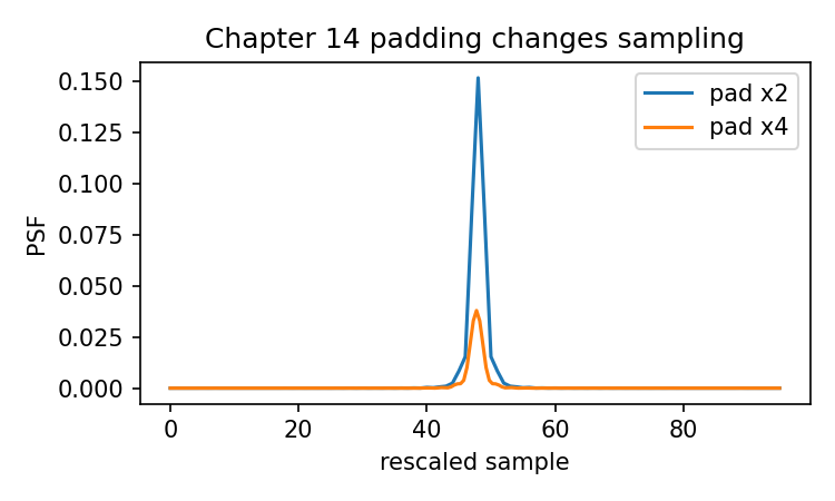
Chapter 15: Merit Function: What the Software Is Actually Optimizing
Optimization is where optical design software can feel most magical.
You change a few settings. You choose some variables. You press an optimization button. The system updates. The spot diagram improves. The MTF rises. The lens looks more “designed” than before.
It is a powerful experience.
It is also easy to misunderstand.
Optimization does not mean the software knows what a good lens is in a human sense. It does not know what you care about unless you express that care numerically. It does not know that a lens should be manufacturable, affordable, compact, bright, stable, elegant, or suitable for a particular sensor unless those requirements appear in the model, constraints, or evaluation targets.
At the numerical level, optimization is usually doing something much plainer:
change variables
→ evaluate a merit function
→ try to make that merit function smaller
That is it.
The difficulty is not that sentence. The difficulty is deciding what the merit function should measure.
A bad merit function can make an optical system “better” in exactly the wrong way.
A good merit function does not replace optical judgment. It encodes optical judgment into numbers carefully enough that an optimizer can work with it.
This chapter opens that calculation.
1. Optimization is not “automatic improvement”
The word “optimize” sounds reassuring. It suggests that the software is moving the design toward some objective good.
But the optimizer does not optimize “goodness.”
It optimizes a defined quantity.
If the quantity is RMS spot radius, the optimizer may reduce RMS spot radius.
If the quantity is wavefront RMS, it may reduce wavefront RMS.
If the quantity is MTF error at selected frequencies and field points, it may improve those selected MTF values.
If the quantity ignores distortion, the optimizer may produce a design with poor distortion.
If the quantity ignores lens thickness, the optimizer may produce an impractical shape.
If the quantity ignores manufacturing tolerance, the optimizer may find a fragile design that only works on paper.
This is the most important sentence in the chapter:
An optimizer follows the merit function, not your intention.
Your intention must be translated into variables, operands, targets, weights, constraints, and bounds.
That translation is optical design work.
The button executes the judgment already encoded in the merit function.
2. What a merit function is
A merit function is a single number that scores a design.
Lower is usually better.
A common least-squares form looks like this:
where:
- is the vector of design variables;
- is the error of the -th evaluation item;
- is the weight of that item;
- is the total merit value.
The function is often an operand error:
where:
- is a computed optical quantity;
- is the target value.
For example:
computed focal length - target focal length
computed RMS spot radius - target RMS spot radius
computed distortion - target distortion
computed MTF at 50 cycles/mm - target MTF
The optimizer does not need to know the emotional meaning of these quantities. It only needs to evaluate , then search for variables that reduce it.
So a merit function is a translation layer:
optical design goals
→ numerical errors
→ weighted sum
→ one scalar score
That scalar score is what the optimizer sees.
3. Variables, operands, targets, weights, bounds
Before writing code, we need a small vocabulary.
Variables
Variables are design parameters the optimizer is allowed to change.
Examples:
- surface radius;
- thickness;
- air gap;
- glass choice;
- aspheric coefficient;
- stop position;
- image plane position;
- lens element spacing.
If a parameter is not variable, the optimizer cannot change it.
This sounds obvious, but it matters. If focus position is fixed, the optimizer cannot refocus. If glass is fixed, it cannot reduce chromatic aberration by choosing another material. If curvatures are fixed, it cannot bend the lens differently.
The optimizer is limited by the variables you give it.
Operands
Operands are measured quantities used in the merit function.
Examples:
- effective focal length;
- RMS spot radius;
- ray intercept error;
- OPD RMS;
- distortion;
- chief ray angle;
- MTF at a selected frequency;
- total track length;
- minimum edge thickness.
An operand is not necessarily a design goal by itself. It becomes part of a goal when paired with a target and weight.
Targets
A target is the desired value for an operand.
Examples:
EFL should be 50 mm
distortion should be 0
RMS spot should be small
MTF at 50 cycles/mm should be high
lens thickness should stay above 1 mm
Some targets are exact. Others are soft preferences.
Weights
Weights tell the optimizer how much each operand matters.
If one operand has a huge weight, the optimizer will try hard to satisfy it, possibly at the expense of others.
If one operand has a tiny weight, the optimizer may largely ignore it.
Weights are not just technical settings. They are design priorities written as numbers.
Bounds
Bounds define allowed ranges.
Examples:
radius must stay between -200 mm and 200 mm
thickness must stay between 1 mm and 20 mm
image plane shift must stay between -2 mm and 2 mm
Bounds prevent the optimizer from escaping into absurd or impossible designs.
Without bounds, an optimizer may find a mathematically convenient solution that no one can manufacture, assemble, or even interpret.
4. A tiny merit function
Let us start with the simplest possible merit function.
Suppose we want a number to become 3.
The error is:
The merit function is:
In code:
def merit_scalar(x):
return (x - 3.0) ** 2
The minimum occurs at:
because then:
This is not optical design yet. But it shows the form.
Now suppose we want two things:
- should be 3;
- should be 10.
Then:
In code:
def merit_two_variables(v):
x, y = v
w1 = 1.0
w2 = 1.0
error_x = x - 3.0
error_y = y - 10.0
return w1 * error_x**2 + w2 * error_y**2
If we increase w2, the optimizer will care more about matching .
This is already the basic structure of many optical merit functions. The only difference is that real operands are not usually simple variables. They are computed from ray tracing, wavefront analysis, PSF, MTF, geometry, and constraints.
5. A simple optimizer loop
Before using SciPy, let us write the most basic optimizer idea by hand.
We will try different values and keep the best one.
import numpy as np
def merit_scalar(x):
return (x - 3.0) ** 2
candidate_values = np.linspace(-10.0, 10.0, 401)
best_x = None
best_m = np.inf
for x in candidate_values:
m = merit_scalar(x)
if m < best_m:
best_m = m
best_x = x
print("Best x:", best_x)
print("Best merit:", best_m)
This brute-force search is slow for high-dimensional problems, but it is honest. It shows what optimization is doing conceptually:
try variable values
compute merit
keep lower merit
A real optimizer is more efficient. It chooses the next trial values intelligently. But it is still trying to reduce a scalar merit function.
This point is worth keeping close. It prevents us from treating optimization as a mysterious intelligence.
6. Using SciPy for minimization
For practical Python examples, we can use scipy.optimize.minimize.
import numpy as np
from scipy.optimize import minimize
def merit_two_variables(v):
x, y = v
w1 = 1.0
w2 = 1.0
error_x = x - 3.0
error_y = y - 10.0
return w1 * error_x**2 + w2 * error_y**2
initial_guess = np.array([0.0, 0.0])
result = minimize(
merit_two_variables,
initial_guess,
method="Nelder-Mead"
)
print(result.x)
print(result.fun)
The result should be close to:
x = 3
y = 10
This is still a toy example. But now we have the same outer shape used in real design scripts:
define variables
define merit function
choose initial guess
call optimizer
inspect result
Optical design adds more expensive calculations inside the merit function.
7. Optimizing focus position
Now let us make the example optical.
We will optimize the image plane position.
This is one of the most understandable optimization problems in optics:
Given a bundle of rays after a lens,
where should the image plane be placed to minimize spot size?
We will use a simplified ray model.
Imagine rays leaving a lens at . Each ray has:
- height ;
- slope .
At an image plane located at distance , the ray height is:
If all rays meet at the same point, the spot is small.
If they land at different heights, the spot is larger.
Let us generate a ray bundle with a little spherical-aberration-like behavior. Marginal rays will focus slightly differently from paraxial rays.
import numpy as np
import matplotlib.pyplot as plt
from scipy.optimize import minimize
def generate_teaching_rays(n_rays=41, pupil_radius=1.0, f0=50.0, spherical=4.0):
"""
Generate a 1D teaching ray bundle after a lens.
Parameters
----------
n_rays : int
Number of rays across the pupil.
pupil_radius : float
Maximum ray height at the lens.
f0 : float
Base paraxial focal distance.
spherical : float
Amount of pupil-dependent focal shift.
Returns
-------
y : 1D array
Ray heights at z=0.
u : 1D array
Ray slopes after the lens.
"""
y = np.linspace(-pupil_radius, pupil_radius, n_rays)
# A simple pupil-dependent focus distance.
# Marginal rays focus at a slightly different distance.
focus_distance = f0 + spherical * y**2
# Slope chosen so each ray would cross y=0 at its own focus distance.
u = -y / focus_distance
return y, u
This is not a full lens model. It is a controlled teaching model.
It gives us rays that do not all share exactly the same focus.
Now define the ray intercept at a candidate image plane:
def ray_heights_at_plane(y, u, z_image):
return y + z_image * u
Define RMS spot radius in this 1D example:
def rms_spot_1d(y_image):
return np.sqrt(np.mean(y_image**2))
The merit function can be RMS spot squared:
def focus_merit(v, y, u):
"""
Merit function for focus optimization.
v[0] is the image plane position.
"""
z_image = v[0]
y_image = ray_heights_at_plane(y, u, z_image)
rms = rms_spot_1d(y_image)
return rms**2
Now run the optimization:
y, u = generate_teaching_rays(
n_rays=41,
pupil_radius=1.0,
f0=50.0,
spherical=4.0
)
initial_guess = np.array([50.0])
result = minimize(
focus_merit,
initial_guess,
args=(y, u),
method="Nelder-Mead"
)
best_focus = result.x[0]
print("Best focus position:", best_focus)
print("Best merit:", result.fun)
The best focus will be near the base focal distance, but not exactly equal to every ray’s focus. Since different pupil zones prefer different focal planes, the optimizer chooses a compromise.
This is already a real optical-design idea:
Best focus is often a compromise, not a place where every ray becomes perfect.
That sentence matters. Optimization often balances competing errors.
8. Plotting merit versus focus
It helps to see the merit function landscape.
z_values = np.linspace(45.0, 58.0, 300)
merit_values = []
for z in z_values:
merit_values.append(focus_merit([z], y, u))
merit_values = np.array(merit_values)
plt.figure(figsize=(6, 4))
plt.plot(z_values, merit_values)
plt.axvline(best_focus, linestyle="--", label="Optimized focus")
plt.xlabel("Image plane position z")
plt.ylabel("Merit: RMS spot squared")
plt.title("Focus merit function")
plt.grid(True)
plt.legend()
plt.tight_layout()
plt.show()
This plot is useful because it removes the mystery.
The optimizer is not “thinking about focus.” It is moving along a curve and looking for a lower value.
For this one-variable case, the merit landscape is simple. Real optical design problems are usually not simple:
- many variables;
- many fields;
- many wavelengths;
- many surfaces;
- nonlinear ray tracing;
- constraints;
- local minima;
- tradeoffs between performance and manufacturability.
But the basic idea is the same.
The optimizer searches a merit landscape.
The merit landscape is created by your optical model and your merit function.
9. Before-and-after spot plot
Let us compare a guessed focus and optimized focus.
def plot_ray_intercepts(y, u, z_before, z_after):
y_before = ray_heights_at_plane(y, u, z_before)
y_after = ray_heights_at_plane(y, u, z_after)
ray_index = np.arange(len(y))
plt.figure(figsize=(7, 4))
plt.plot(ray_index, y_before, "o", label=f"Before: z={z_before:.2f}")
plt.plot(ray_index, y_after, "o", label=f"After: z={z_after:.2f}")
plt.axhline(0.0, linewidth=1)
plt.xlabel("Ray index")
plt.ylabel("Ray height at image plane")
plt.title("Ray intercepts before and after focus optimization")
plt.grid(True)
plt.legend()
plt.tight_layout()
plt.show()
plot_ray_intercepts(
y=y,
u=u,
z_before=50.0,
z_after=best_focus
)
The optimized focus should reduce the spread of ray intercepts.
But notice what it cannot do. It cannot make all rays perfect if the ray bundle contains spherical-aberration-like behavior. Moving the image plane only changes one variable. It cannot remove the underlying aberration.
This is another important lesson:
An optimizer cannot fix an error using a variable that has no power over that error.
If only the image plane can move, the optimizer can refocus. It cannot redesign the lens.
To reduce spherical aberration, it may need curvature changes, aspheric terms, more elements, aperture changes, glass changes, or other variables.
Variable choice defines what the optimizer is capable of doing.
10. Adding weights: paraxial rays versus marginal rays
In optical design, not every ray or operand needs the same weight.
Suppose we care more about central pupil rays than marginal rays. Or suppose we care more about marginal rays because they reveal aperture-related aberrations.
Weights change the compromise.
Let us add ray weights.
def weighted_rms_spot_1d(y_image, weights):
weights = np.asarray(weights)
weights = weights / np.sum(weights)
return np.sqrt(np.sum(weights * y_image**2))
def focus_merit_weighted(v, y, u, weights):
z_image = v[0]
y_image = ray_heights_at_plane(y, u, z_image)
rms = weighted_rms_spot_1d(y_image, weights)
return rms**2
Now create weights that emphasize marginal rays:
pupil_coordinate = y / np.max(np.abs(y))
marginal_weights = 1.0 + 4.0 * pupil_coordinate**2
result_marginal = minimize(
focus_merit_weighted,
initial_guess,
args=(y, u, marginal_weights),
method="Nelder-Mead"
)
best_focus_marginal = result_marginal.x[0]
print("Best focus, equal weights:", best_focus)
print("Best focus, marginal weighted:", best_focus_marginal)
The best focus may shift.
That is not a bug. It is a design priority becoming visible.
Weights are not neutral.
They tell the optimizer what to care about.
This is why copying a merit function without understanding it can be risky. You may also copy someone else’s priorities.
11. Optimizing a thin lens curvature
Now let us optimize something closer to lens design.
We will use the thin lensmaker relation in air:
where:
- is optical power;
- is refractive index;
- is first surface curvature;
- is second surface curvature.
The effective focal length is approximately:
This is a paraxial thin-lens model, not a real thick-lens optimization. It is useful because the variable-operand-target structure is visible.
Suppose we want a 50 mm focal length with glass index .
We can optimize and .
But infinitely many curvature pairs can produce the same power. For example, many combinations of give the same focal length.
So we add a bending preference: keep curvatures moderate.
This creates a merit function with two goals:
- match target focal length;
- avoid unnecessarily strong curvature.
import numpy as np
from scipy.optimize import minimize
def thin_lens_efl(c1, c2, n=1.5):
"""
Thin lens effective focal length in air.
Curvatures are in 1/mm.
Focal length is in mm.
"""
power = (n - 1.0) * (c1 - c2)
if np.abs(power) < 1e-12:
return np.inf
return 1.0 / power
def curvature_merit(v, target_efl=50.0, n=1.5):
"""
Merit function for a toy thin-lens curvature optimization.
Variables
---------
v[0] : c1, first surface curvature [1/mm]
v[1] : c2, second surface curvature [1/mm]
"""
c1, c2 = v
efl = thin_lens_efl(c1, c2, n=n)
# Operand 1: focal length error
efl_error = (efl - target_efl) / target_efl
# Operand 2: curvature penalty
# This discourages extremely curved surfaces.
curvature_penalty = c1**2 + c2**2
w_efl = 100.0
w_bend = 1.0
merit = w_efl * efl_error**2 + w_bend * curvature_penalty
return merit
Now optimize with bounds:
initial_curvatures = np.array([0.02, -0.02])
bounds = [
(-0.1, 0.1), # c1
(-0.1, 0.1), # c2
]
result = minimize(
curvature_merit,
initial_curvatures,
method="L-BFGS-B",
bounds=bounds
)
c1_opt, c2_opt = result.x
efl_opt = thin_lens_efl(c1_opt, c2_opt, n=1.5)
print("Optimized c1:", c1_opt)
print("Optimized c2:", c2_opt)
print("Optimized EFL:", efl_opt)
print("Final merit:", result.fun)
This example is deliberately simple. It is not a substitute for real lens optimization.
But it shows a central design fact:
If the merit function only asks for focal length,
many designs may satisfy it.
Additional operands shape which solution the optimizer prefers.
In real optical design, the merit function may include spot size, wavefront error, distortion, thickness, telecentricity, chief ray angle, MTF, glass constraints, and manufacturability limits.
Those operands are not decorations. They define the design.
12. Constraint versus penalty
There are two common ways to handle design requirements.
Hard constraints
A hard constraint says:
This value must stay inside an allowed range.
For example:
bounds = [
(-0.1, 0.1),
(-0.1, 0.1),
]
The optimizer is not allowed to leave those bounds.
This is useful for variables such as:
- curvature limits;
- thickness limits;
- air gap limits;
- focus travel limits;
- aperture constraints.
Soft penalties
A soft penalty adds cost when something becomes undesirable.
For example:
curvature_penalty = c1**2 + c2**2
This does not forbid curvature. It only discourages large curvature.
Another soft penalty might be:
thickness_penalty = max(0.0, minimum_allowed - thickness)**2
This penalizes thickness below a minimum.
Hard constraints and soft penalties serve different purposes.
Hard constraints define the search region. Soft penalties express preferences inside that region.
A mature merit function often uses both.
13. A merit function is a design argument
It is easy to think of a merit function as a technical file.
It is more than that.
A merit function is an argument about what matters.
If you weight on-axis performance heavily and off-axis performance lightly, you are saying the center of the field matters more.
If you optimize one wavelength only, you are saying color correction is not part of this optimization.
If you target MTF at 10 cycles/mm and 30 cycles/mm but not 80 cycles/mm, you are saying certain detail scales matter more than others.
If you penalize total length, you are saying compactness matters.
If you penalize strong curvature, you are saying manufacturability or sensitivity matters.
The optimizer does not question these choices.
It accepts them.
So when an optimized design surprises you, ask first:
What did I actually ask the optimizer to improve?
Not:
Why did the optimizer fail to understand me?
It understood the merit function exactly enough to follow it.
The merit function may not have understood you.
14. Local minima and starting points
Many optical merit functions are nonlinear.
That means the landscape can have multiple valleys.
An optimizer may find a nearby local minimum instead of a globally best design.
The initial design matters.
This is why optical design often begins from a reasonable starting form:
- a known lens type;
- a paraxial layout;
- a scaled existing design;
- a simple design that already roughly works;
- a designer’s chosen architecture.
Optimization is powerful, but it is not a replacement for choosing a plausible starting structure.
A bad starting point can lead to:
- poor local minimum;
- impossible geometry;
- ray failures;
- extreme curvatures;
- unmanufacturable surfaces;
- unstable designs;
- wasted computation.
A useful practical sentence:
Optimization improves a design inside the design space you give it.
It does not automatically invent the right design space.
This is why Chapter 16 will use a Cooke Triplet rather than asking the optimizer to create a lens from nothing.
A Cooke Triplet is already a meaningful architecture. Optimization can then refine it.
15. Merit functions can fight themselves
Real merit functions contain many operands.
Those operands can conflict.
For example:
- improving edge-field MTF may hurt center performance;
- reducing distortion may increase field curvature;
- reducing spherical aberration may increase coma;
- making the lens faster may worsen aberrations;
- reducing total length may increase surface curvatures;
- improving one wavelength may hurt another.
The optimizer does not solve conflict by wisdom. It solves conflict through the weights and available variables.
If two goals fight, the optimizer finds a compromise according to the merit function.
That compromise may or may not be the design you wanted.
This is why experienced optical designers do not simply press optimize once and accept the result. They inspect the design, adjust the merit function, change variables, add constraints, sometimes change the architecture, then optimize again.
The loop is human and numerical:
define goals
→ optimize
→ inspect result
→ revise goals or variables
→ optimize again
That loop is not a failure of automation. It is how numerical optimization becomes design work.
16. Merit function scale matters
Suppose one operand is measured in millimeters and another is measured in waves.
One error might naturally be around:
0.001
while another might be around:
10
If you square both and add them without scaling, the larger numerical quantity may dominate, even if it is not more important optically.
That is why operands are often normalized.
For example:
This expresses focal length error as a relative error.
For spot size, you might normalize by an allowed value:
For distortion:
Then the merit function becomes easier to interpret:
where each is dimensionless or at least scaled.
Good scaling helps the optimizer and helps the designer.
Poor scaling can make weights misleading.
A weight of 10 means very little if the operands themselves have wildly different natural magnitudes.
17. Optimizing MTF directly
Since we have spent several chapters computing PSF and MTF, it is natural to ask:
Can we put MTF directly into the merit function?
Yes, conceptually.
For example, suppose we want MTF at a certain frequency to be at least 0.5.
A simple penalty could be:
Then:
In code:
def mtf_target_penalty(mtf_value, target=0.5):
error = max(0.0, target - mtf_value)
return error**2
This only penalizes the design if MTF falls below the target.
But direct MTF optimization can be expensive because each merit evaluation may require:
ray tracing
→ OPD or pupil
→ PSF
→ OTF
→ MTF
It can also be noisy or sensitive to sampling choices.
That does not make it wrong. It means we should be careful.
Many optical workflows use a mix of operands:
- ray-based operands for speed and robustness;
- wavefront operands for diffraction-related behavior;
- MTF operands for final image-quality targets;
- geometry operands for manufacturability and packaging.
A practical optimization strategy often starts with simpler operands, then moves toward more image-quality-specific operands later.
The exact strategy depends on the design task.
The important point for this book is simpler:
MTF can be optimized only after it has been computed correctly.
That is why Chapter 14 came before this one.
18. A toy merit function with spot and focal length
Let us combine two optical goals in code.
Suppose we have:
- a focus-position variable;
- a target focus near 50 mm;
- RMS spot should be small;
- focus should not drift too far from the target.
This gives a merit function:
In code:
def focus_merit_with_position_penalty(v, y, u, z_target=50.0):
z_image = v[0]
y_image = ray_heights_at_plane(y, u, z_image)
rms = rms_spot_1d(y_image)
focus_error = (z_image - z_target) / z_target
w_spot = 1.0
w_focus = 0.2
return w_spot * rms**2 + w_focus * focus_error**2
Run it:
result_penalized = minimize(
focus_merit_with_position_penalty,
initial_guess,
args=(y, u),
method="Nelder-Mead"
)
best_focus_penalized = result_penalized.x[0]
print("Best focus without focus penalty:", best_focus)
print("Best focus with focus penalty:", best_focus_penalized)
The result may shift toward the target focus position.
This example shows how merit functions encode tradeoffs.
If the focus penalty is low, the optimizer mostly minimizes spot size.
If the focus penalty is high, the optimizer stays closer to the target focus even if spot size is slightly worse.
Neither is universally right.
It depends on the design goal.
19. Watching the optimization path
For teaching, it is helpful to record the optimizer’s path.
SciPy allows a callback function for many methods.
history = []
def callback(v):
history.append(float(v[0]))
history.clear()
result = minimize(
focus_merit,
initial_guess,
args=(y, u),
method="Nelder-Mead",
callback=callback
)
history = np.array(history)
plt.figure(figsize=(6, 4))
plt.plot(history, "o-")
plt.xlabel("Iteration")
plt.ylabel("Focus position")
plt.title("Optimization path")
plt.grid(True)
plt.tight_layout()
plt.show()
This plot is not usually part of final optical reporting, but it is excellent for learning.
It reminds us that optimization is a sequence of trials, not a single act.
For a simple one-variable problem, the path is easy to understand. For a real lens with many variables, the path is harder to visualize, but the principle remains:
The optimizer repeatedly evaluates designs and moves through variable space.
When an optimization behaves strangely, history can help.
Did it hit a bound? Did it jump to an absurd region? Did merit stop improving? Did variables change wildly? Did one operand improve while another became worse?
Those questions are more useful than simply saying “optimization failed.”
20. What Optiland contributes at this stage
Optiland is valuable here because it connects real optical system data with analysis and optimization tools.
A real optimization workflow does not use our toy generate_teaching_rays() function. It uses an optical system:
surfaces
materials
apertures
fields
wavelengths
variables
analysis operands
optimization method
Conceptually, the Optiland workflow looks like this:
# Version-checked workflow outline.
# Check your installed Optiland version for exact API names.
# 1. Build or load an optical system.
# optic = ...
# 2. Select variables:
# - surface radii
# - thicknesses
# - image plane position
# - aspheric coefficients
# optic.set_variable(...)
# 3. Define merit operands:
# - effective focal length target
# - RMS spot size
# - distortion
# - MTF targets
# - thickness constraints
# merit = ...
# 4. Choose optimizer and settings.
# optimizer = ...
# 5. Run optimization.
# result = optimizer.optimize()
# 6. Analyze before and after:
# - layout
# - spot diagram
# - wavefront
# - PSF
# - MTF
# - geometry constraints
The exact API can change across versions. The concept is stable.
Optiland is not merely pressing an optimization button. It is a Python environment where you can inspect what variables are allowed to change, what operands are included, what weights are used, and how the design changes.
That inspection is the educational value.
A closed workflow may show you the final merit value. An inspectable workflow lets you ask what that value means.
21. A realistic optimization report should show more than merit
A lower merit value is not enough.
After optimization, you should inspect the design from several angles.
At minimum:
before and after layout
before and after prescription
spot diagrams
ray fans
wavefront maps
PSF
MTF
distortion
field curvature
surface curvatures
thicknesses and air gaps
aperture clearances
Why so many?
Because the merit value is compressed.
It can hide which operands improved and which became worse.
A design may reduce RMS spot but increase distortion. It may improve on-axis MTF but hurt field performance. It may improve one wavelength but hurt another. It may look good optically but have impossible thickness.
So do not ask only:
Did the merit go down?
Ask:
Did the design become better for the actual imaging task?
That second question needs optical judgment.
This is another place where software is powerful but not sufficient.
22. Example: reporting operands separately
In our toy focus example, we can report RMS spot before and after.
def report_focus_solution(y, u, z_values):
for label, z in z_values:
y_image = ray_heights_at_plane(y, u, z)
rms = rms_spot_1d(y_image)
print(f"{label}")
print(f" focus position: {z:.6f}")
print(f" RMS spot: {rms:.6f}")
print()
report_focus_solution(
y,
u,
[
("Initial focus", 50.0),
("Optimized focus", best_focus),
("Penalized optimized focus", best_focus_penalized),
]
)
This is better than reporting only the final merit.
For a real lens, you would report each important operand:
EFL error
RMS spot by field
RMS wavefront by field
MTF at selected frequencies
distortion
minimum thickness
total length
A final merit value without operand breakdown is like a final exam score without seeing which questions were missed.
It may be useful, but it is not enough for design understanding.
23. The danger of optimizing the plot you like
Once we know how to compute MTF, it is tempting to optimize until the MTF plot looks better.
That is understandable. But we need to be careful.
A plot is a view of selected data. It may represent:
- one wavelength;
- one field point;
- one focus setting;
- one direction;
- one frequency range;
- one normalization;
- one aperture;
- one sampling condition.
Improving that plot does not automatically improve the whole optical system.
For example, optimizing MTF at one field point may hurt another field point. Optimizing one spatial frequency may not improve another. Optimizing monochromatic MTF may leave chromatic performance poor.
So a safer rule is:
Do not optimize a display.
Optimize a defined set of optical requirements.
The display helps you inspect the result. It should not silently define the whole design goal.
24. Optimization and manufacturability
A purely optical merit function can produce designs that are mathematically attractive but practically unpleasant.
Examples:
- very steep curvatures;
- extremely thin elements;
- tiny air gaps;
- oversized elements;
- strong aspheric departures;
- glass choices that are expensive or unavailable;
- high sensitivity to tolerance;
- surfaces that are difficult to test;
- mechanical packaging conflicts.
Manufacturability is not automatically included in optical performance.
If it matters, it must appear in constraints, bounds, penalties, glass catalogs, tolerance analysis, or later design review.
A lens is not finished because its merit value is low.
A lens is closer to useful when optical performance, mechanical feasibility, manufacturing limits, cost, and tolerance behavior all make sense together.
This book is focused on computation, not full production engineering. Still, the warning belongs here because optimization can easily create overconfidence.
Numerical optimum does not mean practical optimum.
25. Merit function design as a gradual process
In real work, you rarely write the final merit function perfectly on the first try.
A more realistic sequence is:
start with a simple goal
→ optimize
→ inspect failure modes
→ add operands or constraints
→ re-optimize
→ inspect again
For example:
- First target focal length.
- Then reduce on-axis spot.
- Then include off-axis fields.
- Then include multiple wavelengths.
- Then constrain thickness and curvatures.
- Then add distortion targets.
- Then add MTF targets.
- Then check tolerances.
This gradual process is not a sign that the designer is confused. It is how the problem becomes well-defined.
The merit function evolves as you learn what the design tries to do when given freedom.
This is a very practical mindset:
The first merit function reveals the problem.
The later merit functions shape the design.
26. Gradient-based and derivative-free optimization
There are many optimization methods.
At a high level, two families are useful to distinguish.
Derivative-free methods
Methods such as Nelder-Mead do not require gradients.
They can be easy to use and useful for rough problems, but they may become slow as the number of variables grows.
They ask:
If I try nearby points, does the merit get better?
Gradient-based methods
Methods such as L-BFGS-B use derivative information or approximate derivative behavior.
They can be much faster for smooth problems, especially with many variables.
They ask:
Which direction appears to reduce the merit fastest?
Traditional optical design often uses least-squares and damped least-squares-style methods. Modern differentiable optical frameworks can compute gradients through parts of the optical system, which opens the door to more direct gradient-based optimization.
That is the bridge to Chapter 17.
For now, remember the practical distinction:
The optimizer method affects how the search proceeds.
The merit function defines what the search is trying to reduce.
Do not confuse the two.
27. Why optimization belongs after PSF and MTF
This chapter comes after PSF, OTF, MTF, sampling, and normalization for a reason.
If you do not understand the metric, optimizing it is risky.
Suppose your MTF frequency axis is wrong. You may optimize for “50 cycles/mm” while actually evaluating a different frequency.
Suppose your PSF normalization is inconsistent. You may reward energy scaling rather than better image formation.
Suppose your sagittal and tangential directions are mislabeled. You may improve the wrong directional behavior.
Suppose your pupil mask is wrong. You may optimize a square aperture while thinking it is circular.
Optimization amplifies these mistakes.
It does not correct them.
So the safe chain is:
understand the computation
→ verify the metric
→ then optimize the metric
This is not slower in the long run. It prevents elegant nonsense.
28. A complete minimal optimization script
Here is a compact script for the focus optimization example.
It is small enough to run, inspect, and modify.
import numpy as np
import matplotlib.pyplot as plt
from scipy.optimize import minimize
def generate_teaching_rays(n_rays=41, pupil_radius=1.0, f0=50.0, spherical=4.0):
y = np.linspace(-pupil_radius, pupil_radius, n_rays)
focus_distance = f0 + spherical * y**2
u = -y / focus_distance
return y, u
def ray_heights_at_plane(y, u, z_image):
return y + z_image * u
def rms_spot_1d(y_image):
return np.sqrt(np.mean(y_image**2))
def focus_merit(v, y, u):
z_image = v[0]
y_image = ray_heights_at_plane(y, u, z_image)
rms = rms_spot_1d(y_image)
return rms**2
def report_focus_solution(y, u, z_values):
for label, z in z_values:
y_image = ray_heights_at_plane(y, u, z)
rms = rms_spot_1d(y_image)
print(f"{label}")
print(f" focus position: {z:.6f}")
print(f" RMS spot: {rms:.6f}")
print()
def plot_focus_merit(y, u, best_focus):
z_values = np.linspace(45.0, 58.0, 300)
merit_values = np.array([
focus_merit([z], y, u)
for z in z_values
])
plt.figure(figsize=(6, 4))
plt.plot(z_values, merit_values)
plt.axvline(best_focus, linestyle="--", label="Optimized focus")
plt.xlabel("Image plane position z")
plt.ylabel("Merit: RMS spot squared")
plt.title("Focus merit function")
plt.grid(True)
plt.legend()
plt.tight_layout()
plt.show()
def plot_ray_intercepts(y, u, z_before, z_after):
y_before = ray_heights_at_plane(y, u, z_before)
y_after = ray_heights_at_plane(y, u, z_after)
ray_index = np.arange(len(y))
plt.figure(figsize=(7, 4))
plt.plot(ray_index, y_before, "o", label=f"Before: z={z_before:.2f}")
plt.plot(ray_index, y_after, "o", label=f"After: z={z_after:.2f}")
plt.axhline(0.0, linewidth=1)
plt.xlabel("Ray index")
plt.ylabel("Ray height at image plane")
plt.title("Ray intercepts before and after focus optimization")
plt.grid(True)
plt.legend()
plt.tight_layout()
plt.show()
# Build teaching rays
y, u = generate_teaching_rays(
n_rays=41,
pupil_radius=1.0,
f0=50.0,
spherical=4.0
)
# Optimize image plane position
initial_focus = 50.0
result = minimize(
focus_merit,
np.array([initial_focus]),
args=(y, u),
method="Nelder-Mead"
)
best_focus = result.x[0]
# Report
report_focus_solution(
y,
u,
[
("Initial focus", initial_focus),
("Optimized focus", best_focus),
]
)
# Plot
plot_focus_merit(y, u, best_focus)
plot_ray_intercepts(y, u, initial_focus, best_focus)
The code is not the important thing by itself. The structure is.
It has:
variables: image plane position
operand: RMS spot radius
target: as small as possible
merit: RMS spot squared
optimizer: numerical search
report: before and after RMS
That is the skeleton of optical optimization.
Real optical design adds more variables and more operands, but it does not escape this logic.
29. Where this fits in the full computation chain
We can now add optimization to the chain:
lens prescription
→ variables
→ ray tracing / wavefront / PSF / MTF analysis
→ operands
→ merit function
→ optimizer changes variables
→ updated lens prescription
This is not a straight line. It is a loop:
prescription
→ analysis
→ merit
→ variable update
→ new prescription
→ analysis again
That loop repeats until the optimizer stops.
It may stop because:
- merit is low enough;
- improvement becomes small;
- iteration limit is reached;
- variables hit bounds;
- calculation fails;
- the user stops it.
A finished optimization run is not automatically a finished design.
It is a candidate design that must be inspected.
This is the mature way to read optimization output:
The optimizer produced a lower merit value.
Now we must ask what changed, what improved, what worsened, and whether the result still makes optical and practical sense.
30. What this chapter prepares for
Chapter 16 will use a complete example to connect the whole book.
The point will not be merely to show a Cooke Triplet. The point will be to walk through the full computational route:
prescription
→ layout
→ rays
→ spot
→ ray fan
→ OPD
→ pupil function
→ PSF
→ MTF
→ optimization
→ before/after comparison
This chapter gives us the vocabulary needed for that final case study.
When we see an optimized design in Chapter 16, we will know what to ask:
- Which variables were allowed to change?
- Which operands were included?
- What targets were used?
- What weights were used?
- What constraints or bounds were active?
- Did the merit go down?
- Did the optical performance actually improve?
- Did anything become less practical?
- Which plots confirm the improvement?
That is the difference between watching software optimize and understanding optimization.
Chapter summary
Optimization is not automatic optical wisdom. It is numerical search guided by a merit function.
A common least-squares merit function has the form:
where contains design variables, are operand errors, and are weights.
The main pieces are:
variables: what the optimizer may change
operands: what the design evaluates
targets: what values are desired
weights: what matters more or less
bounds: what values are allowed
constraints or penalties: what must be discouraged or prevented
A simple focus optimization can minimize RMS spot size by changing image plane position. A simple thin-lens example can optimize curvatures to match a target focal length while penalizing excessive curvature. These examples are not full lens design, but they expose the mechanism.
The most important practical lesson is:
An optimizer follows the merit function, not your intention.
So the designer’s task is to translate optical goals into a merit function that is accurate, scaled, weighted, bounded, and inspectable.
Optimization belongs after PSF and MTF because bad metrics become worse when optimized. Before optimizing, we must know what the computed quantities mean.
The next chapter will use a complete optical example to bring the whole chain together.
Generated validation figure
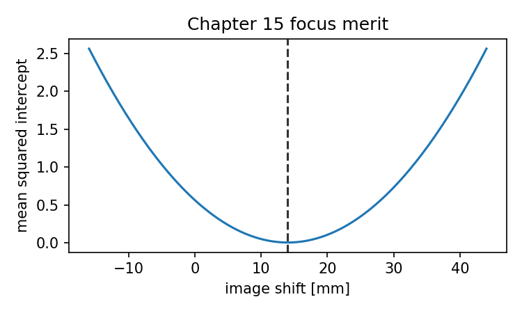
Source and validation note
The least-squares merit function in this chapter is a teaching model. Commercial and research lens-design workflows may use many operand types, constraints, bounds, tolerancing terms, manufacturability penalties, and algorithm choices. The factual claim retained here is narrower: an optimizer follows the explicitly encoded objective and constraints, not an unstated design intention.
Chapter 16: The Cooke Triplet: Walking Through the Whole Computation Chain
A Cooke Triplet is a modest-looking lens.
Three elements. A positive element in front, a negative element in the middle, another positive element behind it. Compared with modern multi-element camera lenses, it looks almost simple.
That simplicity is exactly why it is useful here.
The Cooke Triplet is complicated enough to show real optical behavior:
- spherical aberration;
- coma;
- astigmatism;
- field curvature;
- distortion;
- chromatic correction;
- field-dependent image quality;
- optimization tradeoffs.
But it is still small enough that we can keep the whole design in view.
This chapter uses the Cooke Triplet as a full-chain example. We are not trying to teach every historical or commercial detail of triplet design. We are using it as a test bench.
Here we run the route this book has been building all along:
prescription
→ surfaces and materials
→ ray tracing
→ spot diagram
→ ray fan
→ OPD and wavefront
→ pupil function
→ PSF
→ OTF
→ MTF
→ merit function
→ optimization
→ before/after comparison
If the earlier chapters were individual tools on the table, this chapter is where we use them in sequence.
This is the check: when you see a final MTF curve, can you explain what had to happen before that curve existed?
By the end of this chapter, the answer should be yes.
One note before we start: this chapter uses one fixed teaching prescription instead of treating the Cooke Triplet as a vague placeholder. The numbers are intentionally rounded and pedagogical, not a claim about a historical patent or a production lens. That distinction matters. A fixed teaching prescription is enough to make the calculation chain inspectable. A production prescription would also need glass-catalog validation, tolerance analysis, manufacturability checks, and version-locked engineering review.
1. Why the Cooke Triplet is a good test case
A single thin lens is too simple for a full optical design story. It can show focal length and basic aberration, but it cannot carry much design tradeoff.
A complex modern photographic lens has the opposite problem. It may have many elements, aspheric surfaces, special glasses, floating groups, mechanical constraints, and proprietary design choices. It is realistic, but it is too much for a first full-chain walkthrough.
The Cooke Triplet sits in the useful middle.
It has enough degrees of freedom to make optimization meaningful:
radii
thicknesses
air spaces
glass choices
stop position
image plane position
It has enough aberration behavior to make analysis meaningful:
on-axis and off-axis spot diagrams differ
ray fans show structure
wavefront maps change across field
PSF changes with field and focus
MTF varies by field and direction
And it is small enough that we can still understand the prescription as a table.
That is why lens design education often returns to triplets. They are not toys. They are compact examples of real design logic.
For this book, the Cooke Triplet has one more advantage: it lets us demonstrate the educational value of an open computational workflow.
We can ask not only:
What is the MTF?
but also:
Which prescription produced it?
Which rays were traced?
Which field point was used?
Which wavelength was used?
Which wavefront became the pupil function?
Which PSF produced the OTF?
Which merit function changed the design?
That is the whole point.
2. What we will and will not do
This chapter is a walkthrough, not a full industrial lens design project.
We will not pretend that a few pages of code replace professional optical design software. We will not derive every third-order aberration term. We will not claim that a triplet optimized in a teaching script is ready for manufacturing.
What we will do is more focused:
take one complete lens
run the major analyses
connect each plot to its computational origin
perform a small optimization
compare before and after
That is enough to prove the main promise of the book.
We can now follow a lens from prescription data to image-quality metrics.
The Cooke Triplet is not the protagonist. The computation chain is.
3. The two-track approach in this chapter
We will keep the same two-track method used throughout the book.
Track A: minimal Python understanding
Track A is for understanding the skeleton. It uses small code fragments to show what kind of data is being passed around.
It does not implement a full production ray tracer here. We already built many of those pieces earlier:
- ray representation;
- surface intersection;
- vector refraction;
- pupil sampling;
- OPD to pupil function;
- PSF by FFT;
- OTF and MTF from PSF;
- merit function optimization.
In this chapter, Track A mostly reminds us what each stage means.
Track B: Optiland adapter boundary
Track B is not allowed to be a pile of almost-code. It needs a clean boundary. The book text should show the workflow; the companion code should lock the installed library version and implement a small adapter layer around the actual API.
Read Optiland examples in this chapter in one of two ways:
- Pure Python blocks are meant to be syntactically valid teaching code.
- Adapter sketches describe calls that must be implemented in the companion repository for the pinned Optiland version. They are marked as sketches rather than presented as directly runnable snippets.
A practical companion repository should include:
pyproject.toml
notebooks/16_cooke_triplet_full_chain.ipynb
src/optics_examples/cooke_triplet.py
src/optics_examples/analysis_adapters.py
tests/test_chapter_code_syntax.py
tests/test_cooke_triplet_smoke.py
The contract for the adapter is simple:
make_cooke_triplet() -> optical system object
plot_layout(system) -> layout figure or axis
run_spot_diagram(system, ...) -> spot data and figure
run_ray_fan(system, ...) -> ray-fan data and figure
run_wavefront(system, ...) -> OPD map, pupil mask, metadata
run_psf(system, ...) -> PSF array, coordinate metadata
run_mtf(system, ...) -> frequency axis and MTF curves
optimize_triplet(system, ...) -> optimized system and optimization log
This adapter does not hide the calculation. It prevents the printed book from depending on unstable method names while still requiring the companion code to prove the workflow.
4. The prescription: the lens as data
Before there are plots, there is a prescription.
A lens prescription is not merely documentation. It is the input data for computation.
A simplified triplet prescription might be represented as a table:
| Surface | Radius | Thickness to next | Material | Semi-aperture | Comment |
|---|---|---|---|---|---|
| 0 | Infinity | Object distance | Air | — | Object |
| 1 | Positive | Glass thickness | Crown glass | aperture | Front lens first surface |
| 2 | Negative | Air gap | Air | aperture | Front lens second surface |
| 3 | Negative | Glass thickness | Flint glass | aperture | Middle lens first surface |
| 4 | Positive | Air gap | Air | aperture | Middle lens second surface |
| 5 | Positive | Glass thickness | Crown glass | aperture | Rear lens first surface |
| 6 | Negative | Back focal distance | Air | aperture | Rear lens second surface |
| 7 | Infinity | — | Image | — | Image plane |
For this chapter, we use one fixed teaching prescription. The values below are rounded teaching values in millimeters. They are not presented as a historical Cooke patent prescription, and they are not a manufacturing prescription. Their job is to make the full computation chain concrete.
In code, it may look like this:
from dataclasses import dataclass
from typing import Optional
@dataclass
class SurfaceRecord:
radius: float # mm; use np.inf for plane
thickness: float # mm to next surface
material_after: str # material after this surface
semi_aperture: float # mm
comment: str = ""
cooke_triplet_prescription = [
SurfaceRecord(radius= 23.7, thickness=4.0, material_after="CROWN", semi_aperture=8.0, comment="front element S1"),
SurfaceRecord(radius= -80.0, thickness=6.0, material_after="AIR", semi_aperture=8.0, comment="front element S2"),
SurfaceRecord(radius= -22.0, thickness=2.0, material_after="FLINT", semi_aperture=6.5, comment="middle element S1"),
SurfaceRecord(radius= 22.0, thickness=7.0, material_after="AIR", semi_aperture=6.5, comment="middle element S2"),
SurfaceRecord(radius= 80.0, thickness=4.0, material_after="CROWN", semi_aperture=7.5, comment="rear element S1"),
SurfaceRecord(radius= -23.7, thickness=38.0, material_after="AIR", semi_aperture=7.5, comment="rear element S2"),
]
These numbers are now the fixed teaching prescription for this chapter. A companion repository should keep the same table in machine-readable form, so every figure in this chapter can be regenerated from the same starting data.
The important point is this:
Every later plot begins from this kind of table.
A spot diagram is not drawn from nowhere. A wavefront map is not guessed. An MTF curve is not a software artifact.
They all start from surfaces, distances, materials, apertures, wavelengths, fields, and focus settings.
5. Building or loading the triplet in Optiland
In a pinned Optiland environment, you may either load a sample triplet or build one surface by surface.
The validated companion workflow looks like this:
# Validated wrapper workflow.
# Implemented for optiland==0.6.0 in the companion package.
optic = make_cooke_triplet()
plot_layout(optic)
If building manually, the conceptual steps are:
# Conceptual construction steps.
optic = OpticalSystem()
optic.add_surface(radius=23.7, thickness=4.0, material="CROWN", semi_aperture=8.0)
optic.add_surface(radius=-80.0, thickness=6.0, material="AIR", semi_aperture=8.0)
optic.add_surface(radius=-22.0, thickness=2.0, material="FLINT", semi_aperture=6.5)
optic.add_surface(radius=22.0, thickness=7.0, material="AIR", semi_aperture=6.5)
optic.add_surface(radius=80.0, thickness=4.0, material="CROWN", semi_aperture=7.5)
optic.add_surface(radius=-23.7, thickness=38.0, material="AIR", semi_aperture=7.5)
optic.set_aperture(...)
optic.set_fields(...)
optic.set_wavelengths(...)
optic.set_image_plane(...)
The manuscript package implements the wrapper calls against optiland==0.6.0. If you port the example to another version, rerun the validation tests before trusting the plots.
The structure is what matters:
surfaces first
then aperture
then fields
then wavelengths
then image plane
then analysis
Do not start with MTF. Start with the lens.
6. Choosing fields and wavelengths
A lens does not have one universal performance value.
Performance depends on field point and wavelength.
For a simple triplet example, we might use three fields:
on-axis field
mid field
edge field
and three wavelengths:
blue
green
red
For example:
fields = [
{"name": "axis", "angle_deg": 0.0},
{"name": "mid", "angle_deg": 7.0},
{"name": "edge", "angle_deg": 14.0},
]
wavelengths = [
{"name": "blue", "wavelength_m": 486.1e-9, "weight": 1.0},
{"name": "green", "wavelength_m": 587.6e-9, "weight": 1.0},
{"name": "red", "wavelength_m": 656.3e-9, "weight": 1.0},
]
These are the validation wavelengths used in this manuscript package. A different design goal may require different wavelengths or weights.
A monochromatic design problem is different from a polychromatic imaging problem.
An on-axis-only optimization is different from a field-wide optimization.
A slow lens is different from a fast lens.
So before running analysis, write down the configuration:
What field points?
What wavelengths?
What aperture?
What focus plane?
What performance target?
Without those answers, “the MTF of the lens” is an incomplete phrase.
A better phrase is:
the MTF of this lens at this field, wavelength set, aperture, focus, and direction
It is longer, but it is honest.
7. First plot: the layout
The layout is the first sanity check.
optic = make_cooke_triplet()
plot_layout(
optic,
fields=fields,
wavelengths=wavelengths
)
A layout plot should answer basic questions:
- Are the surfaces in the expected order?
- Are the elements separated correctly?
- Is the stop where you think it is?
- Do rays pass through the clear apertures?
- Does the image plane look roughly plausible?
- Are there obvious ray failures?
The layout is not a performance plot. It does not prove the lens is good.
But it catches large modeling errors early.
If the layout is wrong, every later analysis is suspect.
A good habit is:
Never trust a spot diagram before looking at the layout.
Never trust an MTF curve before looking at the prescription and layout.
This may sound slow. It is faster than debugging a beautiful MTF curve from a broken model.
8. Paraxial check: focal length and f-number
Before real-ray analysis, check the paraxial skeleton.
A triplet is a real lens, but paraxial quantities still matter:
- effective focal length;
- back focal length;
- f-number;
- entrance pupil;
- image distance;
- approximate magnification if finite conjugates are used.
Validated wrapper call:
# Validated wrapper workflow for optiland==0.6.0.
paraxial = optic.paraxial_analysis()
print("Effective focal length:", paraxial.efl)
print("Back focal length:", paraxial.bfl)
print("F-number:", paraxial.f_number)
print("Entrance pupil diameter:", paraxial.entrance_pupil_diameter)
If your intended lens is around 50 mm focal length and the paraxial analysis says 5000 mm, do not continue to PSF.
The paraxial check is the system’s backbone.
It tells you whether the first-order behavior is roughly right before you ask about detailed aberrations.
This connects directly to Chapter 8:
paraxial optics is not old-fashioned decoration;
it is the first consistency check for the whole system.
9. Real ray tracing: where the geometry becomes honest
Now trace real rays.
In a full triplet, real rays do not obey the simple paraxial model exactly. They intersect curved surfaces at real points, refract using local surface normals, and accumulate errors.
Validated wrapper call:
# Validated wrapper workflow for optiland==0.6.0.
ray_bundle = optic.trace_rays(
field=fields[1],
wavelength=wavelengths[1],
pupil_sampling="grid",
num_rays=21,
)
print(ray_bundle.summary())
The real-ray trace is the engine behind many later plots.
From traced rays we can compute:
- spot diagram;
- ray fan;
- transverse aberration;
- chief ray behavior;
- vignetting;
- optical path length;
- wavefront error.
This is why the middle of the book spent so much time on rays.
If ray tracing is wrong, the later wave optics will not be trustworthy.
The computation chain depends on it:
prescription
→ surface intersections
→ refractions
→ ray bundle at image plane
That is the geometric foundation.
10. Spot diagram: the first image-quality view
The spot diagram is often the first visual performance check.
Validated wrapper call:
# Validated wrapper workflow for optiland==0.6.0.
spot_results = run_spot_diagram(
optic,
fields=fields,
wavelengths=wavelengths,
pupil_sampling="grid",
num_rays=21,
)
spot_results.plot()
spot_results.report()
A spot diagram answers:
Where do traced rays land on the image plane?
For the triplet, you should expect field dependence.
The on-axis spot may be relatively compact. Off-axis spots may stretch, tilt, or grow. Different wavelengths may land in slightly different places or have different spreads.
This tells us several things:
- spherical aberration affects the on-axis spot;
- coma and astigmatism appear more strongly off-axis;
- chromatic aberration appears when wavelengths separate;
- focus choice changes the distribution.
But the spot diagram is still ray-based.
It does not show diffraction rings. It does not directly show MTF. It does not replace PSF.
Its role in the chain is:
real ray trace
→ image plane ray intercepts
→ spot diagram
It is a geometric image-quality view.
Useful, but not complete.
11. Reading the spot diagram without overreading it
A compact spot usually suggests better geometric imaging. A large spot suggests more blur.
But there are limits.
A small spot can still be larger than the diffraction-limited Airy disk. A spot smaller than the Airy disk may not matter much because diffraction dominates. A spot diagram near the diffraction limit can be less informative than wavefront, PSF, or MTF.
So for each field, compare spot size to the Airy scale.
A simple calculation:
def airy_radius_um(wavelength_m, f_number):
return 1.22 * wavelength_m * f_number * 1e6
green = 587.6e-9
f_number = 4.0 # example; use paraxial result from the actual system
print("Airy first dark radius [um]:", airy_radius_um(green, f_number))
If the RMS spot radius is much larger than the Airy scale, geometric aberration dominates.
If the spot is comparable to or smaller than the Airy scale, diffraction analysis becomes especially important.
This is a good moment to remember one of the book’s recurring points:
Spot diagrams are computed results, not final truth.
They answer one question well. They do not answer every question.
12. Ray fan: structure inside the spot
A spot diagram shows where rays land. A ray fan shows how ray error changes across the pupil.
Validated wrapper call:
# Validated wrapper workflow for optiland==0.6.0.
ray_fan = run_ray_fan(
optic,
fields=fields,
wavelengths=wavelengths,
pupil_coordinate="normalized",
)
ray_fan.plot()
Ray fans are useful because they reveal structure.
A spot diagram might show a blur cloud. A ray fan can show whether the blur comes from:
- spherical-like behavior;
- coma-like asymmetry;
- astigmatic differences;
- chromatic separation;
- defocus;
- field-dependent imbalance.
This connects to Chapter 9.
A ray fan asks:
How does transverse ray error vary across the pupil?
For a triplet, compare the ray fan at different fields.
On-axis, the fan may show mostly symmetric aberration patterns.
Off-axis, the fan may become asymmetric or direction-dependent.
This is one reason the Cooke Triplet is a good teaching example. It is small, but not boring.
13. Wavefront and OPD: crossing from rays to phase
Now we move from ray intercepts to wavefront error.
The OPD map answers:
At each pupil point, how far ahead or behind is the real wavefront
compared with the reference wavefront?
Validated wrapper call:
# Validated wrapper workflow for optiland==0.6.0.
wavefront = run_wavefront(
optic,
field=fields[1],
wavelength=wavelengths[1],
pupil_sampling=128,
)
opd = wavefront.opd
mask = wavefront.pupil_mask
wavefront.plot_opd(units="waves")
wavefront.report()
The OPD is where the chain changes character.
The spot diagram and ray fan are geometric views. OPD prepares the system for diffraction calculation.
This is the bridge from Chapter 10:
real ray tracing
→ optical path length
→ reference wavefront comparison
→ OPD map
For the triplet, inspect OPD by field.
A good on-axis wavefront may be mostly symmetric. An off-axis wavefront may show coma-like or astigmatic structure. Different wavelengths may show different OPD behavior because refractive index changes.
This is not just another plot. It is the input to the pupil function.
14. Pupil function: encoding the wavefront as complex field
From OPD, we build the pupil function:
This is Chapter 11 returning inside a real lens workflow.
If the Optiland wavefront tool gives us OPD and a pupil mask, the teaching conversion is:
import numpy as np
def pupil_function_from_opd(opd, mask, wavelength, amplitude=None):
if amplitude is None:
amplitude = mask.astype(float)
phase = 2.0 * np.pi * opd / wavelength
pupil = amplitude * np.exp(1j * phase)
pupil[~mask] = 0.0 + 0.0j
return pupil, phase
Then:
pupil, phase = pupil_function_from_opd(
opd=opd,
mask=mask,
wavelength=wavelengths[1]["wavelength_m"],
)
At this point, the Cooke Triplet is no longer only a surface table or ray diagram.
It has become a complex field over the pupil.
That is a major change in representation:
surface prescription
→ ray geometry
→ wavefront error
→ complex pupil function
This is the exact transition that is usually hidden inside analysis software.
Now we can see it.
15. PSF: the point image of the triplet
The PSF is computed from the pupil function:
A minimal implementation is:
def pad_array_centered(array, pad_factor=4):
if pad_factor == 1:
return array
n, m = array.shape
new_n = n * pad_factor
new_m = m * pad_factor
padded = np.zeros((new_n, new_m), dtype=array.dtype)
start_n = (new_n - n) // 2
start_m = (new_m - m) // 2
padded[start_n:start_n + n, start_m:start_m + m] = array
return padded
def compute_psf_from_pupil(pupil, pad_factor=4):
padded = pad_array_centered(pupil, pad_factor=pad_factor)
field = np.fft.fftshift(
np.fft.fft2(
np.fft.ifftshift(padded)
)
)
psf = np.abs(field) ** 2
psf = psf / np.sum(psf)
return psf, field
Then:
psf, image_field = compute_psf_from_pupil(
pupil,
pad_factor=4
)
Optiland may also provide direct PSF analysis:
# Validated wrapper workflow for optiland==0.6.0.
psf_result = run_psf(
optic,
field=fields[1],
wavelength=wavelengths[1],
sampling=128,
padding=4,
)
psf_result.plot(scale="linear")
psf_result.plot(scale="log")
The two-track comparison is educational.
The Optiland PSF is the realistic analysis result. The NumPy PSF shows the computational skeleton.
If they disagree, do not immediately panic. Check:
- same field;
- same wavelength;
- same focus;
- same pupil sampling;
- same aperture mask;
- same OPD sign convention;
- same padding;
- same normalization;
- same coordinate scaling.
That checklist is Chapter 14 doing its job.
16. Reading the triplet PSF
For an on-axis field, a well-corrected triplet may have a compact PSF, but not necessarily a perfect Airy pattern.
For off-axis fields, the PSF may become asymmetric. Energy may move away from the central core. Tails may appear. The log-scale view may reveal faint structure not obvious on linear scale.
Read the PSF in layers:
Central core
Ask:
How concentrated is the main energy?
This relates to sharpness and Strehl-like behavior.
Surrounding structure
Ask:
Where did the energy go?
Rings, tails, and directional spread can matter visually.
Field dependence
Ask:
How does the PSF change from center to edge?
This is critical. A lens can look good on-axis and weak at the edge.
Wavelength dependence
Ask:
Do different wavelengths produce different PSFs or focus positions?
This points toward chromatic behavior.
The PSF is where the lens begins to look like an imaging system rather than only a ray-tracing model.
17. OTF and MTF: the triplet as a frequency response
Now compute OTF and MTF from the PSF:
def compute_otf_mtf(psf):
otf = np.fft.fftshift(
np.fft.fft2(
np.fft.ifftshift(psf)
)
)
center = (otf.shape[0] // 2, otf.shape[1] // 2)
if np.abs(otf[center]) > 0:
otf = otf / otf[center]
mtf = np.abs(otf)
return otf, mtf
Then:
otf, mtf = compute_otf_mtf(psf)
Optiland-style analysis:
# Validated wrapper workflow for optiland==0.6.0.
mtf_result = run_mtf(
optic,
fields=fields,
wavelengths=wavelengths,
frequencies=[10, 20, 40, 80],
directions=["sagittal", "tangential"],
)
mtf_result.plot()
mtf_result.report()
The MTF is now not mysterious.
It is:
PSF
→ Fourier transform
→ OTF
→ magnitude
→ MTF
For the triplet, the MTF curves should vary by field and direction.
A typical pattern might be:
- center field performs better than edge field;
- sagittal and tangential curves separate off-axis;
- higher frequencies drop faster;
- polychromatic MTF may be lower than monochromatic MTF.
The exact result depends on the actual prescription, focus, aperture, and optimization state.
The interpretation should always be tied to configuration.
Do not say:
This is the MTF of the Cooke Triplet.
Say:
This is the MTF for this triplet prescription,
at these fields, wavelengths, aperture, focus setting, and frequency directions.
That is how you avoid overreading the curve.
18. A compact analysis runner
For a real companion repository, it is useful to wrap the full analysis into one function.
The wrapper should not hide the chain. It should organize it.
# Validated adapter structure.
def analyze_triplet(optic, fields, wavelengths):
"""
Run the major analyses for a Cooke Triplet.
This is a workflow outline. The actual implementation should call
the exact API of the pinned optical design library.
"""
results = {}
results["layout"] = plot_layout(
optic,
fields=fields,
wavelengths=wavelengths
)
results["paraxial"] = optic.paraxial_analysis()
results["spot"] = run_spot_diagram(
optic,
fields=fields,
wavelengths=wavelengths
)
results["ray_fan"] = run_ray_fan(
optic,
fields=fields,
wavelengths=wavelengths
)
results["wavefront"] = run_wavefront(
optic,
field=fields[1],
wavelength=wavelengths[1]
)
results["psf"] = run_psf(
optic,
field=fields[1],
wavelength=wavelengths[1]
)
results["mtf"] = run_mtf(
optic,
fields=fields,
wavelengths=wavelengths
)
return results
Then:
before = analyze_triplet(
optic,
fields=fields,
wavelengths=wavelengths
)
The returned dictionary is not just convenient. It forces us to remember that “lens performance” is plural.
There is no single plot that tells the entire story.
A serious before/after comparison should include several views.
19. Before optimization: writing down the diagnosis
Before optimizing, write a short diagnosis.
For example:
Before optimization:
- EFL is close to target but not exact.
- On-axis spot is acceptable.
- Edge field spot is stretched.
- Ray fan shows off-axis asymmetry.
- Wavefront at mid field shows astigmatic structure.
- PSF broadens toward the edge.
- Tangential MTF drops faster than sagittal MTF at higher frequencies.
This diagnosis matters because it tells us what problem we are trying to solve.
If we skip diagnosis and go straight to optimization, we may improve a number without understanding the design.
This is the engineering version of a simple medical rule:
Do not prescribe before diagnosing.
In optical design language:
Do not optimize before deciding what performance failure matters.
For a teaching triplet, a reasonable goal might be:
Improve off-axis image quality while keeping focal length,
reasonable thicknesses, and practical curvatures.
Now we can design the merit function.
20. Choosing variables
A triplet has many possible variables.
For a first optimization, do not release everything.
Start with a controlled set, such as:
selected surface radii
selected air gaps
image plane position
Keep glass fixed at first. Keep semi-apertures fixed. Keep total structure recognizable.
Validated wrapper call:
# Validated wrapper workflow for optiland==0.6.0.
variables = [
optic.surface(1).radius,
optic.surface(2).radius,
optic.surface(3).radius,
optic.surface(4).radius,
optic.surface(5).radius,
optic.surface(6).radius,
optic.gap(2).thickness,
optic.gap(4).thickness,
optic.image_plane.position,
]
for variable in variables:
variable.set_variable(True)
Again, exact API names depend on the library version.
The concept is stable:
The optimizer can only change what you release.
If you do not release image plane position, it cannot refocus.
If you do not release curvatures, it cannot change lens power distribution.
If you release too much too early, the design may become unstable or impractical.
Variable selection is design judgment.
21. Choosing operands
Now define what we want to improve.
A teaching merit function might include:
effective focal length target
RMS spot size across fields
chromatic focus control
distortion control
minimum thickness constraints
curvature penalties
MTF targets at selected frequencies
A simplified merit structure:
Do not add everything at once if you are learning.
A staged optimization is easier to understand:
Stage 1
Hold the lens near the desired first-order layout:
EFL
back focal length
reasonable thicknesses
Stage 2
Improve geometric imaging:
RMS spot
ray aberration
field balance
Stage 3
Improve wave/image-quality metrics:
wavefront RMS
PSF concentration
MTF at selected frequencies
This staged approach is not cowardice. It is clarity.
The optimizer follows the merit function. A staged merit function helps you understand what it is following.
22. The validation merit function
Here is a simplified merit function in pseudocode.
It is not meant to be copied directly into Optiland without adapting API calls. It is meant to show the design logic.
def triplet_merit(optic, fields, wavelengths):
"""
Validation merit function for the Cooke Triplet example.
Lower is better.
"""
merit = 0.0
# 1. First-order target
paraxial = optic.paraxial_analysis()
target_efl = 50.0 # mm
efl_error = (paraxial.efl - target_efl) / target_efl
merit += 100.0 * efl_error**2
# 2. Geometric image quality
for field in fields:
spot = run_spot_diagram(
optic,
fields=[field],
wavelengths=wavelengths,
return_data=True
)
rms_spot_um = spot.rms_radius_um
allowed_spot_um = 20.0
spot_error = rms_spot_um / allowed_spot_um
merit += 1.0 * spot_error**2
# 3. Distortion control
for field in fields[1:]:
distortion_percent = optic.distortion(field=field)
allowed_distortion = 2.0
distortion_error = distortion_percent / allowed_distortion
merit += 0.5 * distortion_error**2
# 4. Geometry penalties
geometry_penalty = optic.geometry_penalty(
min_thickness=1.0,
min_air_gap=0.5,
max_abs_curvature=0.2,
)
merit += 10.0 * geometry_penalty
return merit
This is a validation merit function, not a universal triplet design target.
It is an example of translation:
optical goals
→ computed quantities
→ normalized errors
→ weights
→ scalar merit
A real library may provide built-in merit operands and optimizers, so you may not write the merit function exactly this way. But even then, the logic is the same.
23. Running optimization
Validated Optiland adapter workflow:
# Validated wrapper workflow for optiland==0.6.0.
optimizer_settings = {
"method": "damped_least_squares",
"max_iterations": 100,
"tolerance": 1e-6,
}
optimized_optic, optimization_log = optimize_triplet(
optic,
variables=variables,
merit_function=triplet_merit,
fields=fields,
wavelengths=wavelengths,
settings=optimizer_settings,
)
If using a more general Python optimizer, the structure is:
# Validated adapter structure.
from scipy.optimize import minimize
def pack_variables(optic):
# Extract variable values from the optical system.
...
def unpack_variables(optic, x):
# Write variable values back into the optical system.
...
def merit_from_vector(x, optic, fields, wavelengths):
unpack_variables(optic, x)
return triplet_merit(optic, fields, wavelengths)
x0 = pack_variables(optic)
result = minimize(
merit_from_vector,
x0,
args=(optic, fields, wavelengths),
method="Nelder-Mead",
)
unpack_variables(optic, result.x)
optimized_optic = optic
For real optical design, specialized optimizers and library-native merit functions may be better. The point here is conceptual:
The optimizer changes variables.
Each new design is analyzed.
The merit function scores it.
The optimizer searches for a lower score.
That loop is the engine.
24. After optimization: run the same analyses again
Do not compare before and after using different analysis settings.
Use the same fields, wavelengths, aperture, focus convention, sampling, and plotting scale.
after = analyze_triplet(
optimized_optic,
fields=fields,
wavelengths=wavelengths
)
Now compare.
compare_layout(before["layout"], after["layout"])
compare_spot_diagrams(before["spot"], after["spot"])
compare_ray_fans(before["ray_fan"], after["ray_fan"])
compare_wavefronts(before["wavefront"], after["wavefront"])
compare_psfs(before["psf"], after["psf"])
compare_mtfs(before["mtf"], after["mtf"])
These wrapper names are implemented in the companion validation package for optiland==0.6.0.
The comparison should be disciplined:
same fields
same wavelengths
same frequency axis
same normalization
same display scale
Otherwise, you may be comparing analysis settings rather than lens performance.
25. What improvement might look like
After optimization, you might see:
Prescription
Curvatures have changed, but remain within bounds.
Air spaces have shifted.
Image plane moved slightly.
The triplet shape is still recognizable.
Spot diagram
On-axis spot remains compact.
Mid-field and edge-field spots shrink.
Wavelength separation may reduce.
Some field may improve more than another.
Ray fan
Curves flatten or become more balanced.
Large asymmetric errors reduce.
Residual structure remains, because the design is still a compact triplet.
Wavefront
OPD RMS decreases for selected fields.
Wavefront maps become smoother or less extreme.
Some aberration terms trade against others.
PSF
Central energy becomes more concentrated.
Off-axis PSFs become less stretched.
Log-scale tails may reduce.
MTF
Selected frequencies improve.
Sagittal and tangential curves may move closer together.
Edge-field MTF may rise, especially at mid frequencies.
But not everything improves equally.
That is normal.
Optimization is tradeoff management, not miracle generation.
A mature report says both:
what improved
and:
what did not improve, or what became worse
That honesty is part of technical reliability.
26. A before/after report table
The pinned companion code currently reports this optimization summary:
| Metric | Before | After | Comment |
|---|---|---|---|
| Spot RMS merit [mm^2] | 1.6625847615e-4 | 1.5389416611e-4 | Decreased by 7.44% |
| Optimized variables | R1, R3, R4, R6, BFD | R1, R3, R4, R6, BFD | Bounded L-BFGS-B |
| Iteration count | 0 | 20 | History saved in companion output |
These values come from the pinned optiland==0.6.0 companion run. The merit is the mean squared primary-wavelength RMS spot radius from Optiland SpotDiagram.
The report format matters because the final merit value is insufficient by itself.
It also lets us ask:
- Did the metric we targeted improve?
- Did important untargeted metrics degrade?
- Did geometry remain practical?
- Did field balance improve?
- Did the design become more sensitive?
This is how optimization becomes design review.
27. Why the MTF changed
When the MTF improves, do not stop at the curve.
Ask why.
A possible chain might be:
curvatures changed
→ off-axis ray aberration reduced
→ wavefront OPD reduced
→ PSF energy became more concentrated
→ OTF magnitude increased at selected frequencies
→ MTF curve rose
This is the full-chain explanation.
It is much better than:
The optimizer improved the MTF.
That sentence is true but shallow.
The deeper explanation connects the final metric back to physical and computational causes.
For example:
- If the ray fan became flatter, transverse aberration improved.
- If OPD RMS decreased, phase error decreased.
- If the PSF central core gained energy, point-image concentration improved.
- If the OTF magnitude rose at selected frequencies, contrast transfer improved.
Now the MTF curve is no longer isolated.
It is the last link in a chain you can inspect.
28. When optimization makes something worse
Sometimes the after-design has a lower merit but an ugly surprise.
Examples:
edge thickness becomes too small
distortion increases
one field improves while another worsens
chromatic behavior worsens
surface curvature becomes extreme
MTF improves at one frequency but drops at another
This is not necessarily a software failure.
It may mean the merit function did not include the right penalty, weight, field, wavelength, or constraint.
Return to the merit function.
Ask:
Was the bad behavior measured?
Was it weighted strongly enough?
Was it constrained?
Was the variable space too free?
Was the starting design poor?
Then revise.
For example:
- add a minimum thickness penalty;
- include more field points;
- add wavelength weighting;
- add distortion operands;
- constrain curvature;
- change the optimization stage;
- change the lens architecture if the triplet cannot meet the target.
This is the real loop:
analyze
→ diagnose
→ revise merit function
→ optimize
→ analyze again
The optimizer is not a replacement for that loop. It is one part of it.
29. The Cooke Triplet as a full-chain map
Let us now write the whole triplet workflow as one map.
1. Prescription
surfaces, thicknesses, materials, apertures
2. Configuration
fields, wavelengths, aperture, focus, sampling
3. Paraxial analysis
EFL, BFL, f-number, pupil quantities
4. Real ray tracing
surface intersections, refractions, image-plane intercepts
5. Spot diagram
ray landing distribution by field and wavelength
6. Ray fan
transverse error as a function of pupil coordinate
7. Wavefront / OPD
optical path difference over the pupil
8. Pupil function
amplitude mask and phase from OPD
9. PSF
Fourier transform of complex pupil, squared magnitude
10. OTF
Fourier transform of PSF
11. MTF
magnitude of OTF, sliced by direction and frequency
12. Merit function
weighted errors from chosen operands
13. Optimization
variable update loop to reduce merit
14. Before/after review
compare all relevant plots and constraints
This is the book in one list.
Every item has appeared before. The triplet simply forces them to cooperate.
That cooperation is the real achievement.
30. The full validation script outline
The validation package includes this high-level script structure. The wrapper functions are implemented for optiland==0.6.0 and should be revalidated if the library version changes.
# cooke_triplet_full_chain.py
#
# Validation script outline.
# Wrapper functions are implemented for optiland==0.6.0.
from optics_examples import (
make_cooke_triplet,
set_fields,
set_wavelengths,
plot_layout,
run_paraxial_analysis,
run_spot_diagram,
run_ray_fan,
run_wavefront,
run_psf,
run_mtf,
set_triplet_variables,
build_triplet_merit_function,
run_optimization,
compare_reports,
)
def main():
# 1. Build system
optic = make_cooke_triplet()
# 2. Define configuration
fields = [
{"name": "axis", "angle_deg": 0.0},
{"name": "mid", "angle_deg": 7.0},
{"name": "edge", "angle_deg": 14.0},
]
wavelengths = [
{"name": "blue", "wavelength_m": 486.1e-9, "weight": 1.0},
{"name": "green", "wavelength_m": 587.6e-9, "weight": 1.0},
{"name": "red", "wavelength_m": 656.3e-9, "weight": 1.0},
]
set_fields(optic, fields)
set_wavelengths(optic, wavelengths)
# 3. Analyze before optimization
before = {}
before["layout"] = plot_layout(optic)
before["paraxial"] = run_paraxial_analysis(optic)
before["spot"] = run_spot_diagram(optic, fields, wavelengths)
before["ray_fan"] = run_ray_fan(optic, fields, wavelengths)
before["wavefront"] = run_wavefront(optic, fields, wavelengths)
before["psf"] = run_psf(optic, fields, wavelengths)
before["mtf"] = run_mtf(optic, fields, wavelengths)
# 4. Define variables and merit function
variables = set_triplet_variables(
optic,
vary_radii=True,
vary_air_spaces=True,
vary_image_plane=True,
keep_glass_fixed=True,
)
merit_function = build_triplet_merit_function(
optic,
fields=fields,
wavelengths=wavelengths,
target_efl_mm=50.0,
max_distortion_percent=2.0,
min_thickness_mm=1.0,
mtf_targets=[
{"field": "axis", "frequency_cyc_per_mm": 40, "target": 0.60},
{"field": "edge", "frequency_cyc_per_mm": 40, "target": 0.30},
],
)
# 5. Optimize
optimized_optic, log = run_optimization(
optic,
variables=variables,
merit_function=merit_function,
max_iterations=100,
)
# 6. Analyze after optimization
after = {}
after["layout"] = plot_layout(optimized_optic)
after["paraxial"] = run_paraxial_analysis(optimized_optic)
after["spot"] = run_spot_diagram(optimized_optic, fields, wavelengths)
after["ray_fan"] = run_ray_fan(optimized_optic, fields, wavelengths)
after["wavefront"] = run_wavefront(optimized_optic, fields, wavelengths)
after["psf"] = run_psf(optimized_optic, fields, wavelengths)
after["mtf"] = run_mtf(optimized_optic, fields, wavelengths)
# 7. Compare
compare_reports(before, after, optimization_log=log)
if __name__ == "__main__":
main()
This script is not meant to be a mystery. It is deliberately readable.
Its structure is the full-chain method:
build
→ configure
→ analyze
→ optimize
→ analyze again
→ compare
That is the practical workflow this book has been aiming toward.
31. What to include in the figure set
For this chapter’s final version or companion notebook, include a fixed figure set.
Figure 1: Layout
Purpose:
Show the triplet geometry and ray paths.
Figure 2: Spot diagrams before optimization
Purpose:
Show geometric image quality by field and wavelength.
Figure 3: Ray fans before optimization
Purpose:
Reveal aberration structure across the pupil.
Figure 4: OPD maps
Purpose:
Show wavefront error that will become pupil phase.
Figure 5: PSF before and after
Purpose:
Show how point-image energy distribution changes.
Figure 6: MTF before and after
Purpose:
Show contrast transfer improvement by field and direction.
Figure 7: Prescription change table
Purpose:
Show what the optimizer actually changed.
Figure 8: Operand report
Purpose:
Show which goals improved and which constraints remain limiting.
This figure set prevents the chapter from becoming a pile of disconnected plots.
Each figure has a job.
32. The most important comparison: same settings
When comparing before and after, keep the analysis settings identical.
This matters enough to repeat.
Use the same:
fields
wavelengths
aperture
focus convention
pupil sampling
PSF padding
MTF frequency axis
normalization
plot limits
color scale when possible
If before and after use different settings, the comparison becomes weak.
For example, if the before PSF is shown on a log scale and the after PSF is shown on a linear scale, visual comparison becomes misleading.
If the before MTF uses monochromatic green light and the after MTF uses polychromatic weighting, the curves do not answer the same question.
If the before edge field is 14 degrees and the after edge field is 10 degrees, the improvement may be fake.
A good comparison is boringly strict.
That boring strictness is what makes the result trustworthy.
33. What this chapter proves
This chapter does not prove that the Cooke Triplet is the best lens.
It does not prove that our teaching merit function is production-ready.
It does not prove that every optical problem should be solved with the same workflow.
It proves something more central to the book:
The outputs of optical design software can be connected to a visible computational chain.
The MTF curve is not isolated.
The PSF is not isolated.
The wavefront map is not isolated.
The spot diagram is not isolated.
Each one is produced from earlier data and earlier calculations.
Once you know the chain, you can inspect results more intelligently.
You can ask:
- Is the prescription correct?
- Are the fields and wavelengths appropriate?
- Are the rays traced correctly?
- Is the wavefront reference clear?
- Is the pupil function built with the right phase and mask?
- Is the PSF sampled correctly?
- Is the MTF normalized and labeled correctly?
- Does the merit function measure what we care about?
- Did optimization improve the design or only the score?
These questions are the practical skill.
34. A final walk from MTF back to prescription
Let us practice reading backward.
Suppose the optimized triplet shows improved edge-field tangential MTF at 40 cycles/mm.
Do not stop there.
Walk backward:
MTF improved
→ OTF magnitude improved at that frequency and direction
→ PSF became more favorable for that field
→ pupil phase errors changed
→ OPD map improved
→ ray aberration changed
→ surface curvatures and spacings changed
→ optimizer changed variables according to the merit function
This backward reading is powerful.
It turns a plot into a story of computation and design.
It also helps you challenge the result.
If MTF improved but OPD did not improve, why? If spot improved but MTF did not, why? If the merit went down but edge PSF got worse, what did the merit function ignore?
The ability to ask those questions is the difference between using optical software and understanding optical computation.
35. Where this leaves us
We have now completed the classical computation path promised at the beginning of the book.
The path started with a question:
Where does an MTF curve come from?
Now we can answer in detail.
It comes from an OTF.
The OTF comes from a PSF.
The PSF comes from a complex pupil function.
The pupil function comes from amplitude and phase.
The phase comes from OPD.
The OPD comes from optical path differences computed through the lens.
Those optical paths come from traced rays.
Those rays come from surfaces, materials, wavelengths, fields, and apertures.
And optimization changes the prescription so that selected computed quantities move toward selected targets.
That is the chain.
It is not short. But it is no longer hidden.
The next chapter will look forward. Modern computational optics increasingly wants this whole chain to be differentiable, programmable, and connected to larger imaging systems. That is where automatic differentiation and differentiable ray tracing enter.
But before going there, we needed this chapter.
A differentiable optical system is still an optical system.
If you do not understand the classical chain, automatic differentiation only gives you a faster way to be confused.
Now we have the chain in hand.
Reproducibility checklist for this chapter
The companion code should pass four checks:
1. Rebuild the teaching prescription from the table in this chapter.
2. Generate layout, spot, ray fan, OPD, PSF, and MTF outputs from that same system.
3. Run the before/after analysis with identical field, wavelength, aperture, focus, sampling, normalization, and plotting settings.
4. Replace any illustrative report numbers with values generated by the pinned code.
This is deliberately strict. The chapter is the book's full-chain test. It should feel like an inspection, not like a decorative example.
Chapter summary
The Cooke Triplet is a useful full-chain example because it is small enough to inspect but rich enough to show real optical design behavior.
The complete workflow is:
prescription
→ configuration
→ paraxial analysis
→ real ray tracing
→ spot diagram
→ ray fan
→ OPD / wavefront
→ pupil function
→ PSF
→ OTF
→ MTF
→ merit function
→ optimization
→ before/after comparison
The prescription is the starting data. Fields, wavelengths, aperture, and focus settings define the analysis configuration. Real ray tracing produces spot diagrams and ray fans. Optical path differences produce OPD maps. OPD becomes pupil phase. The pupil function produces the PSF. The PSF produces the OTF and MTF.
Optimization changes selected variables to reduce a merit function. It does not automatically know what “better” means. The merit function defines the target.
A trustworthy before/after comparison must use the same fields, wavelengths, sampling, normalization, and plot settings. A lower merit value is not enough; the design must be inspected through layout, prescription, spots, ray fans, wavefront, PSF, MTF, and geometry constraints.
The main lesson is simple and important:
A final MTF curve is the last visible link in a long computational chain.
This chapter walked through that chain using one complete lens.
Generated validation figures
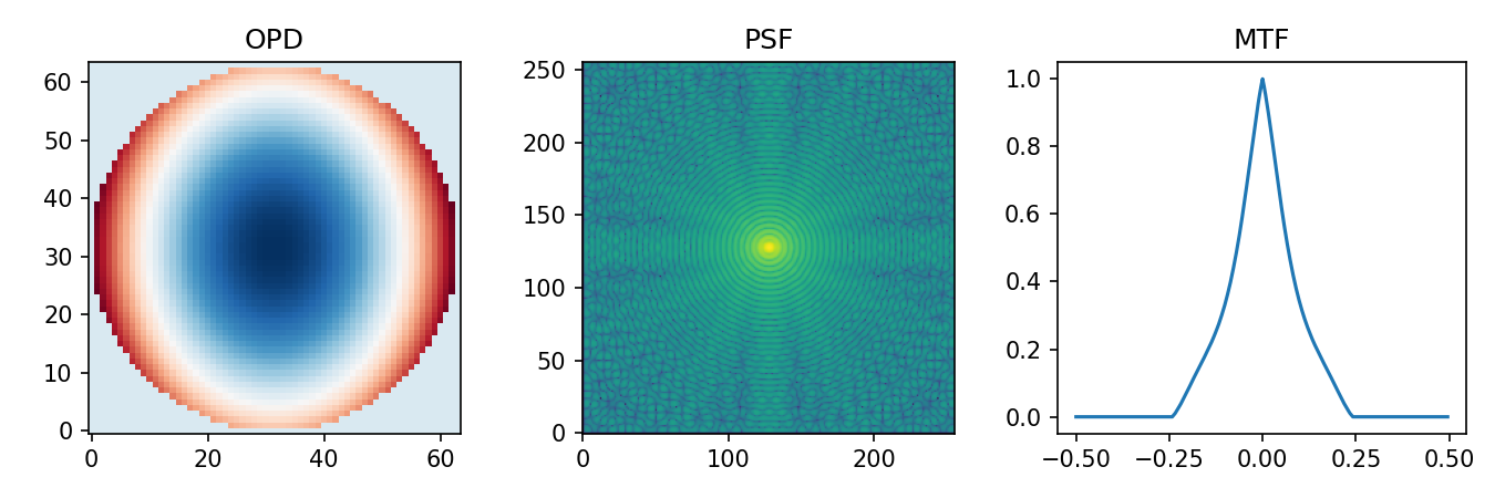
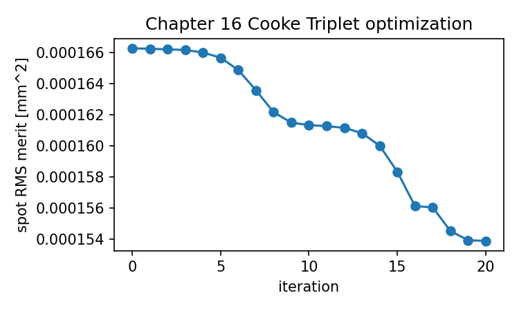
The iteration-level merit history is recorded in ../figures/chapter_16/cooke_optimization_history.csv.
Source and validation note
This chapter is the manuscript's full-chain validation anchor. The reported before/after merit values come from the pinned companion run with optiland==0.6.0; they should not be edited by hand. If the prescription, bounds, variables, fields, wavelengths, sampling, or Optiland version changes, rerun validation and replace both the chapter figures and the recorded merit history.
Chapter 17: Why Differentiable Optics Matters
The previous chapter gave us the classical optical design loop.
We had a prescription. We traced rays. We computed spot diagrams, wavefront maps, PSFs, MTF curves, and a merit function. Then an optimizer changed variables and tried to reduce that merit function.
That loop is already powerful:
lens prescription
→ analysis
→ merit function
→ optimizer
→ updated prescription
But there is a question hiding inside the word “optimizer.”
How does the optimizer know which way to move?
In a simple one-variable focus problem, it can try nearby focus positions and see whether the merit gets better. In a real lens with many radii, thicknesses, aspheric coefficients, materials, and image-quality metrics, blind trial and error becomes expensive.
This is where gradients become important.
A gradient tells us how a result changes when a parameter changes.
For example:
If I slightly increase this surface curvature,
does the RMS spot get better or worse?
If I move this element by 0.01 mm,
does the MTF at 40 cycles/mm rise or fall?
If I change this phase mask parameter,
does the final reconstructed image loss decrease?
Differentiable optics is about making these questions computable.
It does not replace optics. It does not make ray tracing unnecessary. It does not remove the need for physical judgment.
It adds one powerful ability:
The computer can compute not only the optical result,
but also how that result changes with respect to design parameters.
That is the doorway into automatic differentiation, differentiable ray tracing, and modern end-to-end computational imaging.
1. What “differentiable” means here
A function is differentiable if small changes in its input produce changes in its output that can be described by derivatives.
In optical design, we usually have a chain like this:
design parameters
→ ray tracing
→ wavefront
→ PSF
→ image metric
→ loss
A differentiable version of this chain lets us compute:
how the loss changes when each design parameter changes
Mathematically, if the design parameters are collected into a vector:
and the merit or loss is:
then the gradient is:
Each component tells us the local sensitivity of the loss to one variable.
If:
then increasing tends to increase the loss locally.
If:
then increasing tends to decrease the loss locally.
A gradient-based optimizer can use this information to move more intelligently than blind search.
This is the first key idea:
Differentiable optics gives optimization directional information.
The optimizer no longer needs only the value of the merit function. It can also know which variables are pushing the merit up or down.
2. Automatic differentiation is not numerical guessing
There are several ways to estimate derivatives.
One simple method is finite differences.
Suppose we have a function:
We can estimate the derivative by evaluating the function twice:
This is easy to understand, but it has problems:
- it can be slow for many variables;
- it depends on choosing a good ;
- it can be noisy;
- it requires many repeated evaluations;
- it becomes awkward in large computational graphs.
Automatic differentiation, often shortened to autodiff, works differently.
It records the operations used to compute the output, then applies the chain rule through those operations.
If the computation is:
then autodiff computes derivatives through the chain:
This is not symbolic algebra in the traditional sense. It is also not a crude finite-difference estimate. It is derivative computation through the actual executed operations.
Modern machine learning libraries such as PyTorch and JAX are built around this idea.
For optical computation, this matters because our calculations are chains:
radius
→ surface intersection
→ refraction
→ ray position
→ spot size
→ loss
If every step is implemented with differentiable operations, autodiff can compute how the loss changes with respect to the radius.
That is the basic promise.
3. A tiny PyTorch example
Before using optical quantities, let us look at one scalar example.
We want to become 3, so we define:
The derivative is:
At , the derivative is:
That means increasing will reduce the loss.
In PyTorch:
import torch
x = torch.tensor([0.0], requires_grad=True)
loss = (x - 3.0) ** 2
loss.backward()
print("x:", x.item())
print("loss:", loss.item())
print("d loss / d x:", x.grad.item())
The output gradient should be close to:
-6
Now we can do gradient descent manually:
import torch
x = torch.tensor([0.0], requires_grad=True)
learning_rate = 0.1
for step in range(30):
loss = (x - 3.0) ** 2
loss.backward()
with torch.no_grad():
x -= learning_rate * x.grad
x.grad.zero_()
print("optimized x:", x.item())
The variable should move toward 3.
This example is small, but it contains the whole pattern:
define variable
→ compute loss
→ compute gradient
→ update variable
→ repeat
Differentiable optics uses the same pattern, but the loss comes from optical calculations.
4. A differentiable thin lens example
Now let us make the example optical.
We will use a thin lens model in air:
where:
- is optical power;
- is refractive index;
- and are surface curvatures.
The focal length is:
Suppose we want a 50 mm focal length.
We can make and trainable variables.
import torch
# Trainable curvatures in 1/mm
c1 = torch.tensor([0.02], requires_grad=True)
c2 = torch.tensor([-0.02], requires_grad=True)
n = 1.5
target_focal_length = 50.0
optimizer = torch.optim.SGD([c1, c2], lr=0.001)
for step in range(200):
optimizer.zero_grad()
power = (n - 1.0) * (c1 - c2)
focal_length = 1.0 / power
relative_error = (focal_length - target_focal_length) / target_focal_length
curvature_penalty = 0.01 * (c1**2 + c2**2)
loss = relative_error**2 + curvature_penalty
loss.backward()
optimizer.step()
print("c1:", c1.item())
print("c2:", c2.item())
print("focal length:", focal_length.item())
print("loss:", loss.item())
This is a toy model, but it shows the mechanism.
PyTorch computes how the loss depends on and . The optimizer then updates those curvatures.
No finite-difference loop is written by hand.
The computational graph is:
c1, c2
→ optical power
→ focal length
→ focal length error
→ loss
Autodiff computes gradients through that graph.
This is the simplest version of differentiable optical design.
5. A differentiable paraxial ray bundle
The previous example optimized focal length only. Let us move one step closer to imaging.
In paraxial optics, a thin lens changes ray slope approximately as:
where:
- is ray height at the lens;
- is ray angle or slope;
- is focal length.
After propagation by distance , the ray height becomes:
We can build a differentiable ray bundle with PyTorch.
import torch
dtype = torch.float64
# Ray heights at the lens, in mm
y = torch.linspace(-5.0, 5.0, 41, dtype=dtype)
# Incoming collimated rays
u_in = torch.zeros_like(y)
# Trainable lens curvatures and image plane position
c1 = torch.tensor([0.02], dtype=dtype, requires_grad=True)
c2 = torch.tensor([-0.02], dtype=dtype, requires_grad=True)
z_image = torch.tensor([50.0], dtype=dtype, requires_grad=True)
n = 1.5
optimizer = torch.optim.Adam([c1, c2, z_image], lr=0.01)
for step in range(1000):
optimizer.zero_grad()
power = (n - 1.0) * (c1 - c2)
focal_length = 1.0 / power
u_out = u_in - y / focal_length
y_image = y + z_image * u_out
rms_spot = torch.sqrt(torch.mean(y_image**2))
target_focal_length = 50.0
focal_error = (focal_length - target_focal_length) / target_focal_length
curvature_penalty = 0.001 * (c1**2 + c2**2)
loss = rms_spot**2 + 10.0 * focal_error**2 + curvature_penalty
loss.backward()
optimizer.step()
print("c1:", c1.item())
print("c2:", c2.item())
print("z_image:", z_image.item())
print("focal length:", focal_length.item())
print("rms spot:", rms_spot.item())
print("loss:", loss.item())
This is still paraxial and simplified. But it has the structure of differentiable ray optimization:
trainable optical parameters
→ ray calculation
→ image-plane intercepts
→ RMS spot loss
→ gradients
→ parameter update
The gradient tells the optimizer how to change curvatures and image plane position to reduce the loss.
That is the core idea.
6. Why this is different from Chapter 15
In Chapter 15, we used scipy.optimize.minimize on a merit function. That is already optimization.
So what is new here?
The difference is not the existence of a merit function. Both approaches have one.
The difference is how derivative information is obtained and used.
A derivative-free optimizer can evaluate the merit function many times and infer where to search.
A gradient-based differentiable workflow computes the gradient through the optical calculation.
That means we can ask directly:
For large systems, this can be very valuable.
The distinction is:
Traditional merit optimization:
evaluate merit, search for lower values.
Differentiable optimization:
evaluate merit and compute gradients through the calculation.
Both can be useful.
Differentiable optics does not make traditional optimization obsolete. It gives us another set of tools, especially when the optical system is part of a larger differentiable pipeline.
7. Differentiable ray tracing
A differentiable ray tracer is a ray tracer written so that derivatives can flow through its operations.
A normal ray tracer computes:
surface parameters + incoming ray
→ intersection point
→ surface normal
→ refracted direction
→ outgoing ray
A differentiable ray tracer also allows derivatives such as:
how the outgoing ray changes if the surface radius changes
how the image-plane intercept changes if thickness changes
how the loss changes if an aspheric coefficient changes
The ray tracing operations must be differentiable or handled carefully:
- ray-surface intersection;
- surface normal computation;
- refraction;
- propagation;
- optical path length;
- ray intercept error;
- wavefront error.
For a spherical surface, the intersection involves solving a quadratic equation. That solution can be differentiable as long as we stay away from discontinuities such as missed intersections or branch changes.
For a refracted ray, the vector Snell formula can be differentiable as long as we avoid total internal reflection or handle it carefully.
So the differentiable ray tracing chain may look like:
surface radius
→ intersection distance
→ intersection point
→ normal vector
→ refracted direction
→ image-plane intercept
→ loss
→ gradient with respect to radius
This is not conceptually different from the ray tracing we built earlier.
It is the same physics made compatible with gradient computation.
8. A minimal differentiable refraction sketch
Let us sketch the differentiable version of vector normalization and refraction.
This is not a full robust production implementation. It is a teaching fragment.
import torch
def normalize(v, eps=1e-12):
return v / torch.sqrt(torch.sum(v * v, dim=-1, keepdim=True) + eps)
def refract_torch(direction, normal, n1, n2):
"""
Differentiable vector refraction sketch.
direction and normal are tensors with shape (..., 3).
Both should be normalized.
This function assumes no total internal reflection.
"""
direction = normalize(direction)
normal = normalize(normal)
eta = n1 / n2
cos_i = -torch.sum(normal * direction, dim=-1, keepdim=True)
sin_t2 = eta**2 * (1.0 - cos_i**2)
cos_t = torch.sqrt(1.0 - sin_t2)
refracted = eta * direction + (eta * cos_i - cos_t) * normal
return normalize(refracted)
The operations here are PyTorch tensor operations. If direction, normal, or surface parameters used to compute them require gradients, PyTorch can propagate derivatives through this function.
But notice the warning:
This function assumes no total internal reflection.
If:
then the square root becomes invalid for refraction.
A production differentiable ray tracer must handle that case. It may use masks, penalties, alternative branches, or careful domain restrictions.
This is a recurring theme:
Making optics differentiable does not remove optical edge cases.
It makes those edge cases more important.
9. Where differentiability gets difficult
The clean examples above are smooth.
Real optical systems are not always smooth from the optimizer’s point of view.
Several things can create difficulty.
Ray misses and aperture clipping
If a ray passes through an aperture at one parameter value and is blocked at another, the loss can change discontinuously.
The ray is either present or absent.
That is not a smooth change.
Total internal reflection
Refraction can suddenly become impossible when the incidence angle crosses the critical angle.
This creates a branch in the computation.
Surface intersection branch changes
A ray-sphere intersection may have two mathematical roots. Choosing the physically correct one is usually straightforward in ordinary ray tracing, but branch selection can create derivative complications.
Vignetting
Field-dependent ray clipping can introduce hard boundaries.
Small parameter changes may cause rays to appear or disappear.
Glass choice
Selecting a glass from a catalog is discrete. You cannot smoothly differentiate from one glass type to another unless you introduce a continuous proxy model.
Merit functions with hard thresholds
A loss like this is not smooth everywhere:
penalty = max(0.0, value - limit)
It is usable, but the derivative has a kink at the threshold.
FFT magnitude and phase issues
PSF and MTF calculations can be differentiable, but magnitude, normalization, sampling, and phase behavior still need care.
The conclusion is not “differentiable optics is too fragile.”
The conclusion is:
Differentiable optics works best when the computational path is designed with gradients in mind.
That means smooth losses, careful masks, stable parameterizations, and good physical constraints.
10. Smooth losses are often better than hard rules
In Chapter 15, we discussed hard constraints and soft penalties.
Differentiable optimization often prefers smooth penalties when possible.
For example, suppose a thickness should stay above 1 mm.
A hard failure could be:
if thickness < 1.0:
loss = huge_number
This may be useful for rejecting impossible designs, but it gives poor gradient information.
A smoother penalty is:
penalty = torch.relu(1.0 - thickness) ** 2
This penalizes thickness below the limit while giving a gradient when the violation occurs.
For an even smoother version, one can use a softplus-like function:
def soft_lower_bound_penalty(value, lower, sharpness=20.0):
violation = lower - value
return torch.nn.functional.softplus(sharpness * violation) / sharpness
This does not replace hard engineering limits. It gives the optimizer a smoother path while searching.
A good practical pattern is:
Use smooth penalties to guide optimization.
Use hard checks to reject final invalid designs.
This is especially helpful when optimizing optical systems with many variables.
11. Differentiable PSF and MTF
The PSF and MTF computations from earlier chapters can also be part of a differentiable pipeline.
A simplified PyTorch PSF calculation looks like this:
import torch
def pupil_function_torch(opd, mask, wavelength):
phase = 2.0 * torch.pi * opd / wavelength
pupil = mask * torch.exp(1j * phase)
return pupil
def psf_from_pupil_torch(pupil):
field = torch.fft.fftshift(
torch.fft.fft2(
torch.fft.ifftshift(pupil)
)
)
psf = torch.abs(field) ** 2
psf = psf / torch.sum(psf)
return psf
def mtf_from_psf_torch(psf):
otf = torch.fft.fftshift(
torch.fft.fft2(
torch.fft.ifftshift(psf)
)
)
center = (otf.shape[0] // 2, otf.shape[1] // 2)
otf = otf / otf[center]
mtf = torch.abs(otf)
return mtf
If opd depends on trainable parameters, then a loss computed from mtf can send gradients back through:
MTF
→ OTF
→ PSF
→ pupil function
→ OPD
→ optical parameters
That is powerful.
For example, a loss could target high MTF at a selected frequency:
def mtf_loss_at_sample(mtf, fy, fx, target=0.5):
value = mtf[fy, fx]
error = torch.relu(target - value)
return error**2
This is only a sampled teaching example. A real implementation would need correct frequency coordinates, field handling, wavelength handling, sampling, and normalization.
But the idea is clear:
If PSF and MTF are computed with differentiable tensor operations,
they can be used inside gradient-based optimization.
This connects Chapter 13 and Chapter 14 directly to modern optimization.
12. A tiny differentiable phase mask example
Let us build one more example that is closer to computational imaging than classical lens bending.
Suppose we have a pupil with a trainable defocus-like phase coefficient. We want the PSF to concentrate energy at the center.
This is not a full lens design. It is a small differentiable Fourier optics example.
import torch
import matplotlib.pyplot as plt
dtype = torch.float64
device = "cpu"
n = 128
coord = torch.linspace(-1.0, 1.0, n, dtype=dtype, device=device)
yy, xx = torch.meshgrid(coord, coord, indexing="ij")
rho = torch.sqrt(xx**2 + yy**2)
mask_real = (rho <= 1.0).to(dtype)
mask = mask_real.to(torch.complex128)
# Trainable defocus coefficient, measured in waves
defocus_waves = torch.tensor([0.5], dtype=dtype, requires_grad=True)
optimizer = torch.optim.Adam([defocus_waves], lr=0.05)
for step in range(200):
optimizer.zero_grad()
opd_waves = defocus_waves * (2.0 * rho**2 - 1.0)
phase = 2.0 * torch.pi * opd_waves
pupil = mask * torch.exp(1j * phase.to(torch.complex128))
field = torch.fft.fftshift(
torch.fft.fft2(
torch.fft.ifftshift(pupil)
)
)
psf = torch.abs(field) ** 2
psf = psf / torch.sum(psf)
center = (n // 2, n // 2)
# We want to maximize central intensity, so minimize negative peak.
loss = -psf[center]
loss.backward()
optimizer.step()
print("optimized defocus coefficient [waves]:", defocus_waves.item())
print("center intensity:", psf[center].item())
The optimizer should push the defocus coefficient toward a value that increases central PSF energy, typically toward reducing defocus.
This is a tiny example, but it is important because the whole path is differentiable:
phase coefficient
→ pupil phase
→ FFT field
→ PSF
→ center intensity loss
→ gradient
→ phase coefficient update
This is the style of computation that makes modern differentiable optics attractive.
We are no longer limited to optimizing only ray intercepts or simple scalar operands. We can optimize through image formation calculations.
13. End-to-end computational imaging
Classical lens design often treats the lens as the main object.
Modern computational imaging often treats the whole imaging system as the object:
scene
→ optics
→ sensor
→ noise
→ image processing
→ final image or task loss
In an end-to-end differentiable pipeline, some or all of these stages may be differentiable.
That allows a very different kind of optimization.
Instead of asking only:
Does the lens have high MTF?
we can ask:
Does the whole imaging system produce the best final result
after optics, sensor sampling, noise, and reconstruction?
For example, a computational camera may intentionally use an optical element that produces a PSF that looks strange by classical standards, because a reconstruction algorithm can decode it well.
A wavefront coding system may deliberately make the PSF less focus-sensitive.
A metasurface or diffractive optical element may be designed together with a neural reconstruction network.
A lens and image-processing model may be trained together for a specific task.
This is where differentiable optics becomes especially important.
If the whole pipeline is differentiable, we can compute gradients from the final loss all the way back to optical parameters.
The chain becomes:
final image loss
→ reconstruction algorithm
→ sensor model
→ PSF or wave optics model
→ optical parameters
That is end-to-end optimization.
But this power comes with a warning.
If the simulation is unrealistic, the optimized system may perform well in simulation and poorly in reality.
This is sometimes called a simulation-to-reality gap.
For optics, the gap can come from:
- inaccurate material models;
- manufacturing errors;
- alignment tolerances;
- temperature effects;
- sensor noise assumptions;
- diffraction model simplifications;
- polarization effects;
- stray light;
- coating behavior;
- imperfect calibration;
- reconstruction model assumptions.
Differentiability does not remove these problems. It can even hide them behind beautiful training curves.
A careful statement is:
End-to-end differentiable optimization is only as trustworthy as the physical model and loss function it optimizes.
That sentence should stay close whenever the method looks magical.
14. Classical metrics still matter
Differentiable optics can optimize directly for image loss, task loss, or learned perceptual metrics.
That does not make classical optical metrics obsolete.
Spot diagrams, wavefront maps, PSF, MTF, distortion, field curvature, and tolerance analysis still matter because they reveal physical behavior.
A neural reconstruction metric may say the final image looks good, while the optical system has:
- severe field-dependent blur;
- high sensitivity to focus;
- fragile alignment;
- poor color behavior;
- unacceptable distortion;
- low light efficiency;
- strong artifacts outside the training distribution.
Classical metrics are not old furniture to throw away.
They are diagnostic instruments.
A good modern workflow may include both:
classical optical metrics
+
differentiable end-to-end losses
The classical metrics tell us what the optics are doing.
The end-to-end loss tells us how the whole imaging system performs for a specific task.
Those are related but not identical.
This is a mature way to think about differentiable optics:
It expands the design space.
It does not cancel the need to understand optics.
15. Differentiable does not mean physically free
Gradient-based optimization can find surprising designs.
That can be good.
It can also create designs that are hard to manufacture, align, or interpret.
For example, if a phase mask is represented by free pixels, the optimizer may create a highly oscillatory phase pattern. It may perform well in simulation but be impossible to fabricate or too sensitive to wavelength.
If an aspheric surface has many free coefficients, the optimizer may create a surface with large slope changes or difficult testing requirements.
If a material parameter is allowed to vary continuously, the optimizer may choose a refractive index that does not correspond to any real glass.
So the parameterization matters.
A parameterization is how we describe the design variables.
Examples:
surface radii
conic constants
aspheric coefficients
Zernike phase coefficients
freeform surface coefficients
diffractive zone heights
pixelated phase mask values
glass interpolation variables
mechanical spacings
A good parameterization gives the optimizer freedom where freedom is useful and restriction where restriction is necessary.
This is another form of design judgment.
The optimizer follows gradients. It does not know which shapes are manufacturable unless manufacturability appears in the model or constraints.
16. Stable parameterization: an example
Suppose we want to optimize a phase mask.
A tempting parameterization is:
one free phase value per pixel
That gives enormous freedom.
It also allows noisy, rapidly varying patterns.
A smoother alternative is to represent the phase as a sum of low-order polynomial or Zernike-like terms:
Now the trainable variables are coefficients:
This reduces freedom but improves stability and interpretability.
In code, a simple defocus-plus-astigmatism phase model might be:
def phase_model(rho, theta, coeffs):
"""
Simple differentiable phase model.
coeffs[0] : defocus-like term
coeffs[1] : astigmatism-like term
coeffs[2] : coma-like teaching term
"""
defocus = coeffs[0] * (2.0 * rho**2 - 1.0)
astig = coeffs[1] * rho**2 * torch.cos(2.0 * theta)
coma = coeffs[2] * (3.0 * rho**3 - 2.0 * rho) * torch.cos(theta)
return defocus + astig + coma
This is not a full Zernike implementation, but it shows the idea.
The optimizer changes a few meaningful coefficients instead of thousands of unrelated pixels.
That often makes the problem easier and the result more understandable.
A good rule is:
Give the optimizer variables that describe plausible optical changes.
Not merely variables that are easy to put in a tensor.
17. A differentiable loss is a design statement
In Chapter 15, we said a merit function is a design argument.
The same is true here.
A differentiable loss tells the optimizer what matters.
If the loss maximizes PSF center intensity, the optimizer will try to concentrate energy at the center.
If the loss targets MTF at selected frequencies, it will try to improve those frequencies.
If the loss compares a reconstructed image to a ground truth image, it will try to improve that reconstruction.
If the loss is a neural-network task loss, it may optimize for classification or detection performance rather than human visual quality.
None of these is universally right.
The loss must match the imaging task.
For example:
A barcode scanner does not need the same optical priorities as a portrait lens.
A microscope does not need the same priorities as a phone camera.
A star tracker does not need the same priorities as an endoscope.
Differentiable optics does not remove the need to define the task.
It makes the task definition more direct and more consequential.
18. Gradient descent can be fooled
A gradient tells us a local direction.
It does not guarantee a globally best design.
Gradient descent can still suffer from:
- local minima;
- flat regions;
- bad scaling;
- unstable learning rates;
- poor parameterization;
- unrealistic losses;
- constraints not represented in the model;
- sensitivity to initialization.
For example, if the learning rate is too high, optimization may oscillate or diverge.
If the learning rate is too low, it may barely move.
If the initial design is physically poor, rays may miss surfaces or hit invalid regions.
If the loss landscape has many valleys, the optimizer may settle into a local compromise.
So the old lesson remains:
Optimization is a tool, not a guarantee.
Differentiability gives better information. It does not give wisdom.
19. Scaling still matters
Gradients depend on scale.
If one parameter is measured in millimeters and another is a tiny curvature in inverse millimeters, their gradient magnitudes may differ wildly.
If one loss term has values around 1000 and another around 0.001, the large term may dominate.
So differentiable optics still needs:
- normalized variables;
- normalized losses;
- reasonable weights;
- stable units;
- bounded parameters;
- good initialization.
This connects directly to Chapter 14.
Sampling and normalization did not stop mattering because we moved into PyTorch.
They matter more, because the gradients depend on them.
A wrong frequency axis in an MTF loss means the optimizer improves the wrong frequency.
A wrong PSF normalization means the gradient may reward energy scaling instead of image concentration.
A wrong aperture mask means the optimizer designs for the wrong physical system.
The safe chain is:
correct computation
→ correct loss
→ meaningful gradient
→ useful optimization
Do not skip the first two steps.
20. How differentiable optics connects to Optiland
A modern open optical design framework can be valuable in two ways.
First, it can provide classical analysis:
ray tracing
spot diagrams
wavefront
PSF
MTF
optimization
Second, if it supports differentiable or machine-learning-oriented workflows, it can help connect optical models with tensor libraries and gradient-based optimization.
A differentiable workflow outline looks like this:
# Version-checked workflow outline.
# Check the installed Optiland version and companion repository
# for exact API names.
# 1. Build or load an optical system.
# optic = make_system(...)
# 2. Select differentiable backend or tensor mode if supported.
# optic.enable_differentiable_backend("torch")
# 3. Mark parameters as trainable.
# optic.surface(1).radius.requires_grad = True
# optic.surface(2).radius.requires_grad = True
# optic.image_plane.position.requires_grad = True
# 4. Trace rays or compute wave optics result.
# result = optic.trace(...)
# 5. Compute loss.
# loss = result.rms_spot() + mtf_penalty(...)
# 6. Backpropagate.
# loss.backward()
# 7. Optimizer updates parameters.
# optimizer.step()
The exact API may differ. The structure is the important part.
What matters is that optical parameters participate in a differentiable computational graph.
The book’s earlier chain still applies:
surfaces
→ rays
→ wavefront
→ PSF
→ MTF
The differentiable addition is:
loss
→ gradients back through the chain
→ parameter updates
So differentiable optics is not a separate universe. It is the same computation chain with gradients attached.
21. Why open tools matter here
The educational value of open tools becomes especially clear in differentiable optics.
If a tool gives only a final result, you can use the result but cannot easily inspect the computational graph.
If a tool exposes the system as code, you can ask:
- Which parameters require gradients?
- Which operations are differentiable?
- Where are masks or hard branches used?
- Which loss is being optimized?
- How are rays sampled?
- How are invalid rays handled?
- How is the PSF normalized?
- How is the MTF frequency axis defined?
- Which parameters actually changed?
This is not about worshiping open source.
It is about inspectability.
The sharper version of the claim is:
For learning differentiable optics, inspectability is not a luxury.
It is part of understanding the method.
A differentiable pipeline can be even more opaque than a classical one if all you see is a training loss curve.
Open, inspectable code helps prevent that.
22. A small gradient inspection habit
When doing differentiable optics, inspect gradients.
Not every step, not forever, but often enough to catch problems.
For example:
loss.backward()
print("c1 grad:", c1.grad)
print("c2 grad:", c2.grad)
print("z_image grad:", z_image.grad)
Ask:
Are the gradients finite?
Are they extremely large?
Are they exactly zero?
Do they change sign when expected?
Are some variables not receiving gradients?
If a variable has no gradient, perhaps it is not connected to the loss.
If gradients are nan, perhaps a square root, division, invalid ray, or normalization failed.
If gradients are huge, scaling may be poor.
If gradients are tiny, the problem may be flat, saturated, or badly scaled.
This is the differentiable version of inspecting intermediate optical plots.
Just as we inspected pupil amplitude and PSF centering, we inspect gradient health.
A practical debugging checklist:
[ ] Is the loss finite?
[ ] Are gradients finite?
[ ] Do trainable variables actually affect the loss?
[ ] Are units and scaling reasonable?
[ ] Are masks blocking gradients?
[ ] Are hard thresholds creating dead regions?
[ ] Does a small manual parameter change affect the loss as expected?
This saves time.
23. Differentiable optics and MTF: a careful example
Suppose we want to improve MTF at a selected frequency.
A naive loss might be:
loss = -mtf[fy, fx]
This maximizes one MTF sample.
That may work as a toy example, but in real design it is too narrow.
It can encourage the system to improve one point while ignoring nearby frequencies or other fields.
A better teaching loss might average over a small frequency band:
def band_mtf_loss(mtf, fy_slice, fx_slice, target=0.4):
band = mtf[fy_slice, fx_slice]
mean_mtf = torch.mean(band)
error = torch.relu(target - mean_mtf)
return error**2
A still better design loss may include:
multiple fields
multiple wavelengths
multiple frequency bands
geometry penalties
distortion penalties
manufacturing constraints
The differentiable method gives us gradients. It does not choose a wise loss automatically.
The design question remains:
Which image qualities matter for this system?
That question cannot be delegated to autodiff.
24. Differentiable rendering and learned reconstruction
In computational imaging, the optical system may be optimized together with reconstruction software.
A simplified training loop might look like this:
ground truth image
→ optical simulation
→ sensor simulation
→ reconstruction model
→ reconstructed image
→ loss against ground truth
→ gradients update optics and reconstruction parameters
In code structure:
# Conceptual structure only.
for image in training_images:
optimizer.zero_grad()
psf = optical_model(trainable_optical_parameters)
sensor_image = simulate_sensor(image, psf, noise_model)
reconstructed = reconstruction_model(sensor_image)
loss = image_loss(reconstructed, image)
loss.backward()
optimizer.step()
This is much broader than classical lens optimization.
The loss may not be RMS spot or MTF. It may be:
- mean squared image error;
- perceptual loss;
- classification loss;
- detection loss;
- depth estimation loss;
- task-specific reconstruction loss.
This is why differentiable optics matters for modern imaging.
The optical design can be optimized for the final use of the image, not only for classical intermediate metrics.
But again, this is powerful and risky.
If the training images are not representative, the optical system may overfit.
If the sensor model is too clean, the design may fail with real noise.
If manufacturing variation is ignored, the design may be fragile.
If the reconstruction network is too powerful, it may hide optical weaknesses in simulation while producing artifacts in reality.
The more end-to-end the optimization becomes, the more careful the physical validation must be.
25. Validation does not disappear
A differentiable design still needs validation outside the training loop.
For a lens or computational camera, validation may include:
classical optical analysis
independent ray tracing
PSF and MTF checks
tolerance analysis
manufacturing constraints
sensor sampling checks
noise robustness
field and wavelength sweeps
test images outside the training set
physical prototype measurements
If a design only works under the exact differentiable simulation used to train it, it is not yet a robust optical design.
This is a healthy way to view differentiable optics:
Use differentiability to search.
Use optical analysis to understand.
Use validation to trust.
All three are needed.
26. Why this matters to the reader of this book
This book has spent many chapters unpacking classical calculations.
That was not a detour.
It is the foundation needed to understand differentiable optics.
If someone says:
We optimize the lens end to end through a differentiable imaging pipeline.
you can now ask:
- What is the optical model?
- Does it trace real rays or use paraxial approximations?
- Does it include diffraction?
- How is the pupil function represented?
- How is the PSF computed?
- Is the sensor model included?
- What loss is optimized?
- Which optical parameters are trainable?
- Are materials discrete or continuous?
- How are apertures and vignetting handled?
- Are gradients stable?
- What classical metrics were checked afterward?
These are not skeptical questions for their own sake.
They are the questions needed to understand the claim.
Differentiable optics is exciting precisely because it extends the chain we have already built. Without that chain, it is only another black box.
27. A small side-by-side comparison
It may help to compare three optimization styles.
| Style | What it needs | Strength | Risk |
|---|---|---|---|
| Derivative-free search | Merit values | Simple to use; can handle awkward functions | Can be slow; may need many evaluations |
| Classical gradient / least-squares optimization | Merit and derivative-like information | Efficient for smooth optical design problems | Depends on scaling, local behavior, operand design |
| Autodiff differentiable optics | Differentiable computational graph | Can optimize through rays, waves, sensors, and reconstruction | Requires careful differentiable modeling and validation |
None is universally best.
A small lens design problem may work well with traditional optical optimization.
A wavefront-coded computational camera may benefit from end-to-end differentiable optimization.
A rugged engineering design may still need classical tolerance analysis and human review.
The practical lesson is:
Choose the optimization method to match the problem,
not because one method sounds more modern.
28. The main conceptual upgrade
The main upgrade in this chapter is not “use PyTorch.”
The main upgrade is this:
Optical computation can become part of a differentiable program.
Once that happens, optical variables can be optimized together with other differentiable components.
The lens can be connected to:
- phase masks;
- diffractive elements;
- sensor models;
- reconstruction algorithms;
- neural networks;
- task-specific losses.
This is why differentiable optics is important.
It changes the boundary of the design problem.
Classical design often asks:
What lens gives good optical metrics?
Differentiable computational imaging may ask:
What optical system and computational reconstruction together give the best final result?
That is a larger question.
It is also a more dangerous question if asked carelessly.
The larger the optimization loop, the more important it is to understand every link in the chain.
29. What not to believe
Because differentiable optics is connected to machine learning, it is easy for exaggerated claims to appear.
Be cautious with claims like:
The network will learn the optics.
The optimizer will discover the best lens.
Physics constraints are no longer necessary.
MTF is obsolete.
Classical optical design is dead.
These claims are too loose.
A better view is:
Differentiable optimization can search design spaces that are hard to explore manually.
But the result still depends on physical modeling, constraints, losses, data, and validation.
That view keeps the excitement without losing judgment.
This book’s position is not anti-modern. It is anti-mystification.
Differentiable optics is worth learning because it is powerful.
It is also worth demystifying because it is powerful.
30. Preparing for the final chapter
We are now ready to return to the reader’s practical task.
At the beginning of the book, the question was:
Where does an MTF curve come from?
We have answered that.
Now a new question appears:
When optical software gives me any output,
how should I read it?
This includes classical outputs:
- layout;
- prescription;
- spot diagram;
- ray fan;
- OPD;
- PSF;
- MTF;
- merit value.
It also includes modern outputs:
- gradient;
- training loss;
- optimized phase mask;
- differentiable ray trace result;
- end-to-end reconstruction score.
The same habit applies:
Do not stop at the output.
Trace the computation that produced it.
That habit is the real skill this book has been teaching.
The final chapter will collect that skill into a practical reading checklist.
Chapter summary
Differentiable optics means building optical computations so that gradients can be computed with respect to design parameters.
Automatic differentiation applies the chain rule through executed operations. It is different from manually estimating derivatives by finite differences.
A differentiable optical chain may look like:
optical parameters
→ ray tracing or wave optics
→ PSF / MTF / image simulation
→ loss
→ gradients
→ parameter update
PyTorch examples show the basic pattern:
define trainable variables
compute optical result
compute loss
call backward()
update variables
Differentiable ray tracing extends ordinary ray tracing by allowing derivatives to flow through intersections, normals, refraction, propagation, and image-plane errors.
Differentiable PSF and MTF calculations can be built with tensor FFT operations, allowing losses based on image formation or frequency response.
The method is powerful for modern computational imaging because optics, sensors, reconstruction algorithms, and task losses can be optimized together.
But differentiable optics is not magic. It still needs correct physics, stable sampling, meaningful losses, good parameterization, constraints, manufacturability checks, and validation outside the training loop.
The central idea is:
Differentiable optics does not replace the classical computation chain.
It attaches gradients to that chain.
That makes the chain more powerful, but also makes understanding it more important.
Generated validation figure
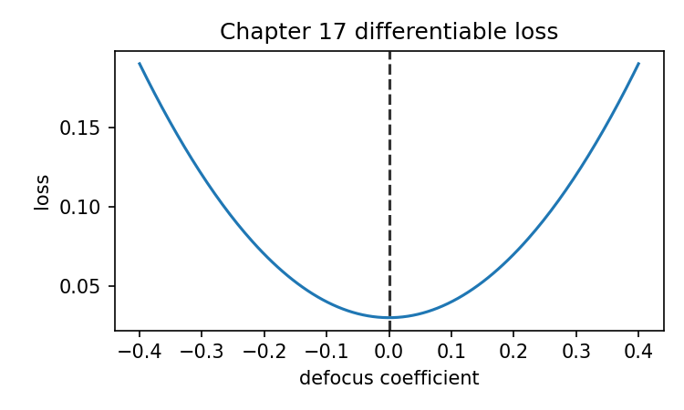
Source and validation note
This chapter is an orientation chapter, not a survey of the entire differentiable-optics literature. The retained claim is limited: automatic differentiation can attach gradients to optical computation chains when the operations are implemented in differentiable numerical frameworks. Practical design still requires physical modeling, constraints, sampling checks, and validation outside the training loop.
Chapter 18: How to Read Optical Software Outputs Now
At the beginning of this book, an MTF curve looked like a finished object.
A piece of software produced it. The curve went down with frequency. There were sagittal and tangential lines. There were field positions, wavelengths, and maybe a diffraction limit. It looked official.
Now we can read that curve differently.
It is no longer a mysterious judgment from the software.
It is the end of a chain:
lens prescription
→ surfaces and materials
→ ray tracing
→ optical path length
→ OPD
→ pupil function
→ PSF
→ OTF
→ MTF
And if optimization is involved, the chain becomes a loop:
prescription
→ analysis
→ merit function
→ optimizer changes variables
→ new prescription
→ analysis again
That is the main change this book wanted to make.
Not that you should stop using optical design software. Quite the opposite. Good optical design software is powerful precisely because it performs so many hard calculations reliably.
You no longer have to treat the output as a sealed verdict.
You can ask where it came from.
You can inspect its inputs.
You can check its assumptions.
You can compare it against the rest of the system.
That is what it means to read optical software outputs well.
1. The first habit: never read a plot alone
A plot is not self-explaining.
A spot diagram, ray fan, wavefront map, PSF, or MTF curve always belongs to a configuration.
Before interpreting any output, ask:
What optical system produced this?
What field point?
What wavelength or wavelength set?
What aperture?
What focus setting?
What sampling?
What normalization?
What coordinate convention?
This may feel slow at first. It is not slow. It is the shortest path to not fooling yourself.
A plot without its configuration is like a number without a unit.
It may look precise, but you do not yet know what it means.
For example, this statement is weak:
The MTF is 0.45.
This statement is better:
At 40 cycles/mm, for the edge field, green wavelength,
tangential direction, full aperture, and current focus setting,
the normalized MTF is 0.45.
It is longer because it is more honest.
Most optical misunderstandings begin when a short statement hides the configuration.
2. Start from the prescription
When you see a software output, do not start by admiring the plot.
Start by asking what prescription produced it.
A lens prescription contains the basic computed object:
surface radius
thickness
material
semi-aperture
conic or aspheric terms
stop position
image plane
This is not paperwork. It is the system.
Every later calculation depends on it.
A practical reading sequence is:
1. Prescription
2. Layout
3. Paraxial properties
4. Real ray analysis
5. Wavefront analysis
6. PSF / MTF
7. Optimization report
If the prescription is wrong, every later output is downstream of that error.
So the first check is plain:
Does this model represent the optical system I think it represents?
Look for simple mistakes:
- radius sign errors;
- wrong glass;
- thickness in the wrong unit;
- missing stop;
- wrong image distance;
- semi-aperture too small;
- surface order mistake;
- wavelength definition mismatch;
- fields entered in the wrong unit.
These are not glamorous errors. They are common.
Optical computation is full of advanced mathematics, but many bad results begin with ordinary bad input.
3. Then look at the layout
The layout is the first visual sanity check.
It tells you whether the prescription has become a plausible physical system.
Ask:
Do the elements appear in the right order?
Do rays pass through the aperture?
Does the stop appear where expected?
Do rays reach the image plane?
Are there obvious ray failures?
Does the scale look reasonable?
The layout does not prove image quality. A bad lens can have a perfectly reasonable layout.
But an obviously wrong layout makes later plots untrustworthy.
This is a useful rule:
Do not trust a beautiful MTF curve from a lens layout you have not checked.
The layout is the first defense against hidden modeling mistakes.
4. Use paraxial results as the skeleton check
Paraxial analysis is not old-fashioned decoration. It is the skeleton of the optical system.
Before reading detailed image-quality plots, check:
effective focal length
back focal length
f-number
numerical aperture
pupil diameter
magnification
chief ray behavior
These are first-order quantities. They tell you whether the system is roughly the lens you intended to build.
If you expected a 50 mm lens and the paraxial analysis gives 500 mm, do not continue interpreting the PSF. Something is wrong upstream.
If you expected f/4 and the computed aperture behaves like f/16, your diffraction scale and MTF cutoff will be different.
If the entrance pupil is not where you expect, field behavior and aperture sampling may surprise you.
The paraxial result is not the final truth. Real rays will depart from it.
But it gives the reference frame.
Paraxial analysis tells you the optical system’s first-order identity.
Real ray analysis tells you how reality departs from that identity.
Read them in that order.
5. Spot diagrams: read them as ray intercept statistics
A spot diagram is not a drawing of blur in the wave-optical sense.
It is a distribution of ray intercepts at an image plane.
It answers:
Where do sampled rays land?
When reading a spot diagram, ask:
Which field point is this?
Which wavelengths are included?
How were pupil rays sampled?
Is the spot shown relative to the chief ray, centroid, or ideal image point?
What is the scale bar?
Is the Airy disk shown?
The Airy disk comparison is especially useful.
If the geometric spot is much larger than the Airy disk, geometric aberration is probably important.
If the geometric spot is much smaller than the Airy disk, diffraction may dominate, and spot size alone may not tell the whole story.
Do not overread a spot diagram near the diffraction limit.
A spot diagram can be very useful, but it is still geometric.
It does not show diffraction rings.
It does not directly show contrast transfer.
It does not replace PSF or MTF.
A careful reading is:
This spot diagram shows the geometric landing pattern of sampled rays
for this field, wavelength set, aperture, and image plane.
That sentence keeps the plot in its proper place.
6. Ray fans: look for structure, not only size
A ray fan shows ray error as a function of pupil coordinate.
It answers:
How does ray error vary across the pupil?
This makes it more diagnostic than a spot diagram in many cases.
When reading a ray fan, ask:
Is the curve symmetric or asymmetric?
Does it show spherical-like behavior?
Does it show coma-like behavior?
Do tangential and sagittal fans differ?
Do different wavelengths separate?
Does the fan flatten after optimization?
A spot diagram may show a cloud. The ray fan can show why the cloud has that shape.
Use it as a structural diagnostic.
For example:
- a symmetric fan on-axis may suggest spherical aberration or defocus-like behavior;
- an asymmetric fan off-axis may suggest coma-like behavior;
- different tangential and sagittal behavior may point toward astigmatism;
- color-separated fans point toward chromatic effects.
The ray fan is not just another plot.
It is one of the best ways to see how real rays depart from the ideal reference.
7. Wavefront and OPD: ask what reference is being used
OPD is the bridge between ray optics and diffraction imaging.
It answers:
How far ahead or behind is each pupil point compared with a reference wavefront?
When reading an OPD or wavefront plot, ask:
What is the reference wavefront?
What wavelength is used?
Are units shown in length or waves?
Is piston removed?
Is tilt removed?
Is defocus removed?
What pupil coordinates are used?
Is the pupil vignetted or clipped?
These questions matter.
The same physical wavefront can look different depending on whether piston, tilt, or defocus has been removed. That does not mean the software is lying. It means wavefront plots are referenced quantities.
OPD in meters or micrometers is a physical path difference.
OPD in waves is normalized by wavelength:
So a wavefront error that is small in micrometers may still be large in waves at short wavelength.
This is why units matter so much.
A good reading habit is:
Before interpreting a wavefront map, identify the wavelength, reference, removed terms, and pupil definition.
Only then decide what the map says.
8. Pupil function: remember amplitude and phase
The pupil function combines aperture amplitude and wavefront phase:
When a software tool computes PSF or MTF by diffraction, something equivalent to this representation is usually involved.
So when reading a diffraction result, ask:
What aperture mask was used?
Is there vignetting?
Is the amplitude uniform?
Is there apodization?
What OPD produced the phase?
Which wavelength was used?
What sign convention is used?
This matters because PSF changes do not only come from wavefront aberration.
They can also come from pupil amplitude:
- central obstruction;
- vignetting;
- aperture clipping;
- apodization;
- transmission variation;
- diffractive or phase elements.
A clear aberrated lens may have uniform amplitude but nonuniform phase.
An obstructed system may have flat phase but nonuniform amplitude.
Both affect the PSF.
Do not read every PSF feature as “aberration.” Some features are aperture structure.
9. PSF: read it as energy distribution
The PSF answers:
What image-plane intensity distribution does one ideal point produce?
When reading a PSF plot, ask:
Is the display linear or logarithmic?
Is the PSF normalized by energy or peak?
What is the image-plane coordinate unit?
What field and wavelength does it represent?
Is it monochromatic or polychromatic?
Is the central peak centered?
Is the plot cropped?
What is the sampling?
Linear and logarithmic PSF displays tell different visual stories.
A linear plot emphasizes the central energy concentration.
A log plot reveals weak rings, tails, and halos.
Neither is “the true one.” They are two displays of the same data.
Read both when possible.
Also distinguish energy normalization from peak normalization.
Energy normalization:
is useful for comparing how energy is distributed.
Peak normalization:
is useful for comparing shapes visually.
But peak-normalized PSFs cannot be used directly for Strehl comparison because the peak has already been forced to one.
A careful PSF reading is:
Where is the point-source energy going,
under this field, wavelength, aperture, focus, sampling, and normalization?
That is the question the PSF answers.
10. MTF: read it as a selected view of frequency response
MTF is the magnitude of the OTF:
It answers:
How strongly does the system transfer contrast at different spatial frequencies?
But a plotted MTF curve is usually not the whole 2D MTF.
It is a selected slice or set of slices.
When reading an MTF curve, ask:
What field point?
What wavelength or wavelength weighting?
What aperture?
What focus?
What direction: sagittal, tangential, radial, horizontal, vertical?
What frequency unit?
Is it diffraction MTF or geometric MTF?
Is it normalized to 1 at zero frequency?
What frequency range matters for the application?
The direction question is important.
Sagittal and tangential directions are defined relative to field geometry. They are not automatically the same as horizontal and vertical array slices unless the coordinate system is known.
The frequency unit is also important.
Cycles/mm, cycles/degree, and normalized frequency are not interchangeable.
A curve that looks strong on a normalized axis may not mean what you think at a sensor’s pixel pitch.
A better MTF reading habit is:
Do not ask only whether the curve is high.
Ask high at which frequency, for which field, in which direction, and under which wavelength and focus condition.
That is the difference between reading the curve and merely looking at it.
11. Always connect MTF back to PSF
MTF can feel abstract. When it does, walk backward.
MTF
← OTF
← PSF
← pupil function
← OPD
← ray tracing
← prescription
If MTF is low at high frequency, ask:
What does the PSF look like?
If sagittal and tangential MTF separate, ask:
Does the PSF or ray fan show directional blur?
If edge-field MTF is weak, ask:
What do the spot diagram, ray fan, and OPD map show at the edge field?
The MTF curve is powerful because it summarizes contrast transfer. It is limited because it compresses the spatial structure of blur.
Use it with PSF.
A healthy reading pair is:
PSF shows where point energy goes.
MTF shows how contrast survives by spatial frequency.
If you keep those two views together, MTF becomes much less mysterious.
12. Read optimization output as a before/after argument
When software says a design has been optimized, do not ask only:
Did the merit value go down?
Ask:
What variables changed?
What operands were included?
What targets were used?
What weights were used?
What constraints or bounds were active?
What improved?
What worsened?
What stayed unmeasured?
The merit value is a compressed score.
A lower merit value means the optimizer reduced the defined objective. It does not automatically mean the design is better in every meaningful way.
A careful optimization report should show:
prescription before and after
layout before and after
operand table before and after
spot diagrams
ray fans
wavefront maps
PSFs
MTFs
geometry constraints
This may seem like a lot. It is the minimum needed to understand what happened.
The optimizer follows the merit function, not your intention.
So after optimization, read the result as an argument:
The design changed in these ways.
These metrics improved.
These constraints remained acceptable.
These metrics did not improve or were not checked.
Therefore the design is better for this defined task.
That is much stronger than:
The optimized lens has lower merit.
13. Read differentiable optics outputs the same way
Differentiable optics adds gradients, but it does not remove the need for interpretation.
When reading a differentiable optimization result, ask:
What parameters were trainable?
What loss was optimized?
What physical model was used?
Were rays, wave optics, sensor sampling, and reconstruction included?
Were constraints smooth, hard, or absent?
Were gradients finite and stable?
Was the result validated outside the training loss?
A decreasing training loss is not a complete optical argument.
It is only one piece of evidence.
If a phase mask, freeform surface, or computational camera has been optimized end-to-end, still ask for classical checks:
PSF
MTF
field behavior
wavelength behavior
tolerance
manufacturability
sensor sampling
noise robustness
out-of-distribution images
Differentiable optics is exciting because it attaches gradients to the optical chain.
But the chain still needs to be physically meaningful.
A safe reading habit is:
Use gradients to search.
Use optical analysis to understand.
Use validation to trust.
That sentence is worth keeping.
14. The full reading checklist
Here is a practical checklist you can use when reading optical software outputs.
A. System definition
[ ] What is the lens prescription?
[ ] Are units clear?
[ ] Are surface signs correct?
[ ] Are materials correct?
[ ] Is the aperture stop defined?
[ ] Are semi-apertures or clear apertures reasonable?
[ ] Is the image plane where expected?
[ ] Are fields and wavelengths defined?
B. Layout and first-order checks
[ ] Does the layout look physically plausible?
[ ] Do rays pass through the expected apertures?
[ ] Are there ray failures?
[ ] Is effective focal length close to expectation?
[ ] Is f-number or NA correct?
[ ] Are pupil quantities plausible?
[ ] Is magnification, if relevant, correct?
C. Ray-based analysis
[ ] Which field and wavelength does the spot diagram show?
[ ] Is the scale clear?
[ ] Is the Airy disk shown or separately computed?
[ ] Does the ray fan explain the spot shape?
[ ] Are sagittal and tangential behaviors separated?
[ ] Is chromatic separation visible?
D. Wavefront analysis
[ ] What OPD reference is used?
[ ] Are piston, tilt, or defocus removed?
[ ] Are units in waves or length?
[ ] What wavelength is used?
[ ] Is the pupil mask clear?
[ ] Does the OPD pattern match the ray fan diagnosis?
E. PSF analysis
[ ] Was the PSF computed from a complex pupil function or another method?
[ ] Is it monochromatic or polychromatic?
[ ] Is the display linear or logarithmic?
[ ] Is normalization energy-based or peak-based?
[ ] Is the coordinate axis physical, angular, or pixel-based?
[ ] Is sampling adequate?
[ ] Does the Airy scale make sense?
F. MTF analysis
[ ] Is MTF computed from PSF / OTF or by another approximation?
[ ] Is it normalized at zero frequency?
[ ] What is the frequency unit?
[ ] Which field points are shown?
[ ] Which wavelengths or weights are used?
[ ] Which directions are shown?
[ ] Does the cutoff frequency make sense?
[ ] Are curves compared under identical settings?
G. Optimization analysis
[ ] What variables were released?
[ ] What operands were used?
[ ] What targets and weights were assigned?
[ ] What bounds and constraints were active?
[ ] Did the merit value decrease?
[ ] Which individual operands improved?
[ ] Did any important metric worsen?
[ ] Did geometry remain practical?
[ ] Was the result checked outside the optimized metrics?
This checklist is not meant to make you cautious to the point of paralysis.
It is meant to keep your confidence attached to evidence.
15. A shorter emergency checklist
When you have very little time, use this shorter version.
1. What system and configuration produced this output?
2. What exact quantity is plotted?
3. What are the units and normalization?
4. What assumptions or references are used?
5. What upstream calculation produced it?
6. What other plot should confirm or challenge it?
7. What would make this interpretation false?
The last question is especially useful.
A strong interpretation should be falsifiable.
For example:
Interpretation:
Edge MTF is low because off-axis astigmatism is spreading the PSF.
Checks:
Ray fan should show tangential/sagittal separation.
OPD should show field-dependent astigmatic structure.
PSF should be directionally spread.
If those checks fail, revise the interpretation.
This is how you move from plot reading to optical reasoning.
16. A small output-reading template
For your own work, you can write a short report for each major plot.
Use this template:
Output:
Configuration:
Input data:
Computation path:
Units and normalization:
Main observation:
Cross-check:
Limitation:
Next action:
For example:
Output:
Chapter 16 Cooke Triplet optimization report.
Configuration:
Three-field, three-wavelength Cooke Triplet analysis with the pinned optiland==0.6.0 companion code.
Input data:
Cooke Triplet prescription, selected radii and back focal distance as optimization variables.
Computation path:
Prescription -> ray tracing -> spot RMS merit -> bounded L-BFGS-B optimization.
Units and normalization:
Spot RMS merit in mm^2. The merit is lower when the selected-field RMS spot radii are lower.
Main observation:
The Chapter 16 companion run reduced spot RMS merit from 1.6625847615e-4 to 1.5389416611e-4, a 7.44% decrease.
Cross-check:
The optimization history is recorded in figures/chapter_16/cooke_optimization_history.csv, and the merit plot is recorded in figures/chapter_16/cooke_merit_optimization.png.
Limitation:
This run proves that the bounded optimization path executes and lowers the defined merit. It does not replace a full design acceptance review.
Next action:
Inspect layout, spots, ray fans, wavefront, PSF, MTF, and geometry constraints before accepting the design.
This kind of report may feel verbose at first. It is very effective.
It forces the output to sit inside the computation chain.
17. What you can now do
If you have followed the book, you now have several concrete abilities.
You can read a lens prescription
You know that a lens prescription is a data structure:
surfaces
radii
thicknesses
materials
apertures
aspheric terms
image plane
You know this is where computation begins.
You can trace one ray conceptually
You know a ray has an origin, direction, wavelength, and sometimes intensity or polarization state.
You know it propagates as:
You know it intersects surfaces and refracts according to surface normals and refractive indices.
You can understand real versus paraxial rays
You know paraxial optics gives the first-order skeleton.
You know real rays reveal aberrations.
You know both matter.
You can interpret spot diagrams and ray fans
You know spot diagrams are ray intercept distributions.
You know ray fans show error structure across the pupil.
You know neither is the same as a diffraction PSF.
You can understand OPD and wavefront error
You know OPD connects geometric path calculation to wave phase.
You know OPD must be interpreted with wavelength, reference wavefront, and removed terms in mind.
You can build a pupil function
You know the pupil function is:
You know it combines aperture amplitude and phase.
You can compute PSF from the pupil function
You know the PSF comes from the squared magnitude of a Fourier-transformed pupil field:
You know sampling, padding, centering, and normalization matter.
You can compute MTF from PSF
You know:
You know the MTF curve is often a slice through a 2D frequency response.
You can understand optimization
You know a merit function is usually a weighted sum of operand errors.
You know variables, targets, weights, bounds, and constraints define what the optimizer can do.
You know lower merit is not automatically better design.
You can understand differentiable optics at the right level
You know differentiable optics attaches gradients to the optical computation chain.
You know autodiff can optimize through rays, waves, sensors, and reconstruction models if the computational path is differentiable.
You also know that gradients do not remove the need for physics, constraints, sampling, and validation.
That is a substantial toolkit.
18. What you should not conclude
It is just as important to know what this book has not claimed.
This book does not make you a professional optical designer by itself.
It does not replace years of design experience, manufacturing knowledge, tolerance analysis, stray light control, coating design, optomechanics, or system engineering.
It does not say minimal Python scripts are enough for production work.
It does not say Optiland or any open-source tool should blindly replace mature commercial tools in every engineering environment.
It does not say MTF is bad.
It does not say classical optical design is obsolete.
The claim is more specific and more useful:
If you can see the computation chain behind optical software outputs,
you can learn faster, debug better, and trust results for better reasons.
That is the promise.
19. How to continue learning
There are several natural next paths.
Path 1: Deeper geometrical optics
Study more complete aberration theory:
third-order aberrations
pupil aberration
field curvature
distortion
chromatic correction
stop shift effects
This will make ray fans and wavefront maps more meaningful.
Path 2: Fourier optics
Go deeper into:
coherent imaging
incoherent imaging
partial coherence
pupil autocorrelation
sampling theory
transfer functions
phase transfer
This will make PSF, OTF, and MTF feel less like isolated formulas.
Path 3: Optical design practice
Work through actual lens examples:
singlet
doublet
Cooke Triplet
Tessar-like forms
microscope objective simplifications
telephoto or wide-angle layouts
Analyze before optimizing. Then optimize. Then compare.
Path 4: Numerical methods
Study:
root finding
least squares
gradient descent
automatic differentiation
conditioning
local minima
parameter scaling
This will make optimization less mysterious.
Path 5: Computational imaging
Explore:
wavefront coding
diffractive optics
phase masks
sensor models
deconvolution
learned reconstruction
end-to-end differentiable design
This is where classical optics and modern computation meet.
Choose one path based on what you want to build.
The foundation from this book should help with all of them.
20. The final return to the MTF curve
Let us return to the original curve.
Imagine you are looking at an MTF plot now.
The old way to read it was:
The curve is high or low.
The lens is good or bad.
The new way is:
This curve is a selected slice through the magnitude of the OTF.
The OTF came from the Fourier transform of the PSF.
The PSF came from the complex pupil function.
The pupil function encoded aperture amplitude and OPD phase.
The OPD came from optical path differences through the system.
Those paths came from traced rays.
Those rays came from a prescription, materials, fields, wavelengths, aperture, and focus setting.
That is a much longer reading.
But it is also much more useful.
Now you can ask:
Which field is weak?
Which direction is weak?
Which frequency matters?
Is the weakness visible in the PSF?
Does the wavefront explain it?
Does the ray fan show the aberration structure?
Can optimization improve it?
What would be the cost of improving it?
The curve is no longer an endpoint.
It is a doorway back into the system.
That is the practical transformation this book was designed to create.
21. The quiet confidence of knowing the chain
There is a particular kind of confidence that comes from understanding a computation chain.
It is not the confidence of memorizing names.
It is not the confidence of pressing a button and hoping the software is right.
It is not the confidence of pretending complex things are simple.
It is quieter than that.
It sounds like this:
I may not know every detail yet,
but I know what inputs this result needs,
what calculation produced it,
what assumptions it depends on,
and what I should check next.
That is enough to keep going.
Optical design is full of detail. No single book removes that.
But once the chain is visible, detail becomes navigable.
You can place each new concept somewhere:
Is this about the prescription?
Is this about ray tracing?
Is this about paraxial structure?
Is this about aberration?
Is this about wavefront?
Is this about diffraction?
Is this about sampling?
Is this about optimization?
Is this about validation?
That map is the real outcome of the book.
22. The final checklist of capability
Here is the ending capability list promised by the blueprint.
After this book, you should be able to:
[ ] Read a basic lens prescription as a computational data table.
[ ] Explain how a ray is represented in code.
[ ] Describe how a ray intersects and refracts at a surface.
[ ] Understand why real rays differ from paraxial rays.
[ ] Interpret focal length, f-number, NA, and other first-order quantities.
[ ] Explain what a spot diagram computes.
[ ] Explain what a ray fan reveals.
[ ] Explain what OPD and wavefront error mean.
[ ] Convert OPD into pupil phase.
[ ] Build a complex pupil function from amplitude and phase.
[ ] Explain how a PSF is computed from the pupil function.
[ ] Explain how OTF and MTF are computed from the PSF.
[ ] Check sampling, normalization, FFT shift, and frequency-axis issues.
[ ] Understand what a merit function is.
[ ] Read optimization output as a before/after design argument.
[ ] Understand what automatic differentiation adds to optical optimization.
[ ] Ask better questions when optical software gives you a plot.
You do not need to be perfect at all of these immediately.
None of them should feel like magic anymore.
23. A final word on tools
This book used Optiland as an open reference point because open tools make the computation easier to inspect.
But the main character was never one tool.
The main character was the chain.
Commercial software, open-source libraries, and your own teaching scripts can all be valuable when you know what to ask of them.
A mature attitude toward tools is:
Use powerful software.
Respect its complexity.
Check its inputs.
Understand its outputs.
Reproduce small pieces when you need to learn.
Do not confuse the interface with the calculation.
That is the balance.
You do not need to rebuild every optical design tool from scratch.
But rebuilding small pieces teaches you what the tool is doing.
Once you have done that, the software output becomes less intimidating and more informative.
That is exactly where we wanted to arrive.
Chapter summary
This final chapter turned the book’s computation chain into a reading method for optical software outputs.
The central rule is:
Never read a plot alone.
Read the system, configuration, computation path, units, normalization, and assumptions behind it.
A lens output should be traced back through:
prescription
→ layout
→ paraxial analysis
→ real ray tracing
→ spot diagram and ray fan
→ OPD and wavefront
→ pupil function
→ PSF
→ OTF
→ MTF
→ merit function and optimization
Spot diagrams show ray intercepts. Ray fans show error structure across the pupil. OPD shows wavefront error relative to a reference. The pupil function encodes amplitude and phase. PSF shows point-source energy distribution. MTF shows contrast transfer by spatial frequency. Optimization changes variables to reduce a defined merit function. Differentiable optics attaches gradients to this same chain.
The final answer to the opening question is now clear:
An MTF curve is not from a software button.
It is the final visible result of a long optical computation chain.
Once you can see that chain, you can read optical software outputs with more patience, more skepticism, and more confidence.
Generated validation figure
Companion Code
The repository contains the tested implementations used to check the manuscript's numerical claims and generate its figures. The package supports Python 3.10 through 3.13 and pins Optiland 0.6.0.
Set up the environment
Install uv, clone the repository, and run:
uv sync --locked
uv run pytest -q
The tests cover pure optical calculations, the pinned Optiland adapter, Python blocks in the manuscript, generated figures, and the complete Cooke Triplet example.
Regenerate validation figures
uv run python scripts/generate_chapter_validation.py
This command intentionally rewrites the shared figures/ directory and writes validation reports under validation/. It is for maintainers; readers do not need to run it to build the book.
Browse the implementation in src/optics_examples.
Sources and Further Reading
The book uses the following primary references for stable optical principles, material data, numerical methods, and version-specific software behavior.
Software and validation
- Optiland 0.6.0 on PyPI — pinned package metadata and Python requirements.
- Optiland documentation — feature orientation; the live documentation is not the versioned API contract for this book.
- The repository's tests and generated figures — manuscript-specific numerical evidence.
Geometrical optics and lens design
- Warren J. Smith, Modern Optical Engineering.
- Warren J. Smith, Modern Lens Design.
- Rudolf Kingslake and R. Barry Johnson, Lens Design Fundamentals.
- John E. Greivenkamp, Field Guide to Geometrical Optics.
Fourier optics and image quality
- Joseph W. Goodman, Introduction to Fourier Optics.
- Max Born and Emil Wolf, Principles of Optics.
- Virendra N. Mahajan, Optical Imaging and Aberrations.
Materials and numerical computation
- SCHOTT optical glass data.
- Mikhail N. Polyanskiy, “Refractiveindex.info database of optical constants,” Scientific Data 11, 94 (2024).
- refractiveindex.info.
- Jorge Nocedal and Stephen J. Wright, Numerical Optimization.
- PyTorch documentation.