Chapter 15: Merit Function: What the Software Is Actually Optimizing

Optimization is where optical design software can feel most magical.

You change a few settings. You choose some variables. You press an optimization button. The system updates. The spot diagram improves. The MTF rises. The lens looks more “designed” than before.

It is a powerful experience.

It is also easy to misunderstand.

Optimization does not mean the software knows what a good lens is in a human sense. It does not know what you care about unless you express that care numerically. It does not know that a lens should be manufacturable, affordable, compact, bright, stable, elegant, or suitable for a particular sensor unless those requirements appear in the model, constraints, or evaluation targets.

At the numerical level, optimization is usually doing something much plainer:

change variables
→ evaluate a merit function
→ try to make that merit function smaller

That is it.

The difficulty is not that sentence. The difficulty is deciding what the merit function should measure.

A bad merit function can make an optical system “better” in exactly the wrong way.

A good merit function does not replace optical judgment. It encodes optical judgment into numbers carefully enough that an optimizer can work with it.

This chapter opens that calculation.

1. Optimization is not “automatic improvement”

The word “optimize” sounds reassuring. It suggests that the software is moving the design toward some objective good.

But the optimizer does not optimize “goodness.”

It optimizes a defined quantity.

If the quantity is RMS spot radius, the optimizer may reduce RMS spot radius.

If the quantity is wavefront RMS, it may reduce wavefront RMS.

If the quantity is MTF error at selected frequencies and field points, it may improve those selected MTF values.

If the quantity ignores distortion, the optimizer may produce a design with poor distortion.

If the quantity ignores lens thickness, the optimizer may produce an impractical shape.

If the quantity ignores manufacturing tolerance, the optimizer may find a fragile design that only works on paper.

This is the most important sentence in the chapter:

An optimizer follows the merit function, not your intention.

Your intention must be translated into variables, operands, targets, weights, constraints, and bounds.

That translation is optical design work.

The button executes the judgment already encoded in the merit function.

2. What a merit function is

A merit function is a single number that scores a design.

Lower is usually better.

A common least-squares form looks like this:

$$M(\mathbf{x}) = \sum_i w_i f_i(\mathbf{x})^2$$

where:

• $\mathbf{x}$ is the vector of design variables;
• $f_i(\mathbf{x})$ is the error of the $i$-th evaluation item;
• $w_i$ is the weight of that item;
• $M(\mathbf{x})$ is the total merit value.

The function $f_i$ is often an operand error:

$$f_i(\mathbf{x}) = q_i(\mathbf{x}) - t_i$$

where:

• $q_i(\mathbf{x})$ is a computed optical quantity;
• $t_i$ is the target value.

For example:

computed focal length - target focal length
computed RMS spot radius - target RMS spot radius
computed distortion - target distortion
computed MTF at 50 cycles/mm - target MTF

The optimizer does not need to know the emotional meaning of these quantities. It only needs to evaluate $M$, then search for variables $\mathbf{x}$ that reduce it.

So a merit function is a translation layer:

optical design goals
→ numerical errors
→ weighted sum
→ one scalar score

That scalar score is what the optimizer sees.

3. Variables, operands, targets, weights, bounds

Before writing code, we need a small vocabulary.

Variables

Variables are design parameters the optimizer is allowed to change.

Examples:

• surface radius;
• thickness;
• air gap;
• glass choice;
• aspheric coefficient;
• stop position;
• image plane position;
• lens element spacing.

If a parameter is not variable, the optimizer cannot change it.

This sounds obvious, but it matters. If focus position is fixed, the optimizer cannot refocus. If glass is fixed, it cannot reduce chromatic aberration by choosing another material. If curvatures are fixed, it cannot bend the lens differently.

The optimizer is limited by the variables you give it.

Operands

Operands are measured quantities used in the merit function.

Examples:

• effective focal length;
• RMS spot radius;
• ray intercept error;
• OPD RMS;
• distortion;
• chief ray angle;
• MTF at a selected frequency;
• total track length;
• minimum edge thickness.

An operand is not necessarily a design goal by itself. It becomes part of a goal when paired with a target and weight.

Targets

A target is the desired value for an operand.

Examples:

EFL should be 50 mm
distortion should be 0
RMS spot should be small
MTF at 50 cycles/mm should be high
lens thickness should stay above 1 mm

Some targets are exact. Others are soft preferences.

Weights

Weights tell the optimizer how much each operand matters.

If one operand has a huge weight, the optimizer will try hard to satisfy it, possibly at the expense of others.

If one operand has a tiny weight, the optimizer may largely ignore it.

Weights are not just technical settings. They are design priorities written as numbers.

Bounds

Bounds define allowed ranges.

Examples:

radius must stay between -200 mm and 200 mm
thickness must stay between 1 mm and 20 mm
image plane shift must stay between -2 mm and 2 mm

Bounds prevent the optimizer from escaping into absurd or impossible designs.

Without bounds, an optimizer may find a mathematically convenient solution that no one can manufacture, assemble, or even interpret.

4. A tiny merit function

Let us start with the simplest possible merit function.

Suppose we want a number $x$ to become 3.

The error is:

$$f(x)=x-3$$

The merit function is:

$$M(x)=(x-3)^2$$

In code:

def merit_scalar(x):
    return (x - 3.0) ** 2

The minimum occurs at:

$$x=3$$

because then:

$$M(3)=0$$

This is not optical design yet. But it shows the form.

Now suppose we want two things:

• $x$ should be 3;
• $y$ should be 10.

Then:

$$M(x,y)=w_1(x-3)^2+w_2(y-10)^2$$

In code:

def merit_two_variables(v):
    x, y = v

    w1 = 1.0
    w2 = 1.0

    error_x = x - 3.0
    error_y = y - 10.0

    return w1 * error_x**2 + w2 * error_y**2

If we increase w2, the optimizer will care more about matching $y=10$.

This is already the basic structure of many optical merit functions. The only difference is that real operands are not usually simple variables. They are computed from ray tracing, wavefront analysis, PSF, MTF, geometry, and constraints.

5. A simple optimizer loop

Before using SciPy, let us write the most basic optimizer idea by hand.

We will try different values and keep the best one.

import numpy as np


def merit_scalar(x):
    return (x - 3.0) ** 2


candidate_values = np.linspace(-10.0, 10.0, 401)

best_x = None
best_m = np.inf

for x in candidate_values:
    m = merit_scalar(x)

    if m < best_m:
        best_m = m
        best_x = x

print("Best x:", best_x)
print("Best merit:", best_m)

This brute-force search is slow for high-dimensional problems, but it is honest. It shows what optimization is doing conceptually:

try variable values
compute merit
keep lower merit

A real optimizer is more efficient. It chooses the next trial values intelligently. But it is still trying to reduce a scalar merit function.

This point is worth keeping close. It prevents us from treating optimization as a mysterious intelligence.

6. Using SciPy for minimization

For practical Python examples, we can use scipy.optimize.minimize.

import numpy as np
from scipy.optimize import minimize


def merit_two_variables(v):
    x, y = v

    w1 = 1.0
    w2 = 1.0

    error_x = x - 3.0
    error_y = y - 10.0

    return w1 * error_x**2 + w2 * error_y**2


initial_guess = np.array([0.0, 0.0])

result = minimize(
    merit_two_variables,
    initial_guess,
    method="Nelder-Mead"
)

print(result.x)
print(result.fun)

The result should be close to:

x = 3
y = 10

This is still a toy example. But now we have the same outer shape used in real design scripts:

define variables
define merit function
choose initial guess
call optimizer
inspect result

Optical design adds more expensive calculations inside the merit function.

7. Optimizing focus position

Now let us make the example optical.

We will optimize the image plane position.

This is one of the most understandable optimization problems in optics:

Given a bundle of rays after a lens,
where should the image plane be placed to minimize spot size?

We will use a simplified ray model.

Imagine rays leaving a lens at $z=0$. Each ray has:

• height $y$;
• slope $u$.

At an image plane located at distance $z$, the ray height is:

$$y_\text{image}=y+zu$$

If all rays meet at the same point, the spot is small.

If they land at different heights, the spot is larger.

Let us generate a ray bundle with a little spherical-aberration-like behavior. Marginal rays will focus slightly differently from paraxial rays.

import numpy as np
import matplotlib.pyplot as plt
from scipy.optimize import minimize


def generate_teaching_rays(n_rays=41, pupil_radius=1.0, f0=50.0, spherical=4.0):
    """
    Generate a 1D teaching ray bundle after a lens.

    Parameters
    ----------
    n_rays : int
        Number of rays across the pupil.
    pupil_radius : float
        Maximum ray height at the lens.
    f0 : float
        Base paraxial focal distance.
    spherical : float
        Amount of pupil-dependent focal shift.

    Returns
    -------
    y : 1D array
        Ray heights at z=0.
    u : 1D array
        Ray slopes after the lens.
    """
    y = np.linspace(-pupil_radius, pupil_radius, n_rays)

    # A simple pupil-dependent focus distance.
    # Marginal rays focus at a slightly different distance.
    focus_distance = f0 + spherical * y**2

    # Slope chosen so each ray would cross y=0 at its own focus distance.
    u = -y / focus_distance

    return y, u

This is not a full lens model. It is a controlled teaching model.

It gives us rays that do not all share exactly the same focus.

Now define the ray intercept at a candidate image plane:

def ray_heights_at_plane(y, u, z_image):
    return y + z_image * u

Define RMS spot radius in this 1D example:

$$\mathrm{RMS}=\sqrt{\frac{1}{N}\sum_j y_j^2}$$

def rms_spot_1d(y_image):
    return np.sqrt(np.mean(y_image**2))

The merit function can be RMS spot squared:

def focus_merit(v, y, u):
    """
    Merit function for focus optimization.

    v[0] is the image plane position.
    """
    z_image = v[0]

    y_image = ray_heights_at_plane(y, u, z_image)

    rms = rms_spot_1d(y_image)

    return rms**2

Now run the optimization:

y, u = generate_teaching_rays(
    n_rays=41,
    pupil_radius=1.0,
    f0=50.0,
    spherical=4.0
)

initial_guess = np.array([50.0])

result = minimize(
    focus_merit,
    initial_guess,
    args=(y, u),
    method="Nelder-Mead"
)

best_focus = result.x[0]

print("Best focus position:", best_focus)
print("Best merit:", result.fun)

The best focus will be near the base focal distance, but not exactly equal to every ray’s focus. Since different pupil zones prefer different focal planes, the optimizer chooses a compromise.

This is already a real optical-design idea:

Best focus is often a compromise, not a place where every ray becomes perfect.

That sentence matters. Optimization often balances competing errors.

8. Plotting merit versus focus

It helps to see the merit function landscape.

z_values = np.linspace(45.0, 58.0, 300)
merit_values = []

for z in z_values:
    merit_values.append(focus_merit([z], y, u))

merit_values = np.array(merit_values)

plt.figure(figsize=(6, 4))
plt.plot(z_values, merit_values)
plt.axvline(best_focus, linestyle="--", label="Optimized focus")
plt.xlabel("Image plane position z")
plt.ylabel("Merit: RMS spot squared")
plt.title("Focus merit function")
plt.grid(True)
plt.legend()
plt.tight_layout()
plt.show()

This plot is useful because it removes the mystery.

The optimizer is not “thinking about focus.” It is moving along a curve and looking for a lower value.

For this one-variable case, the merit landscape is simple. Real optical design problems are usually not simple:

• many variables;
• many fields;
• many wavelengths;
• many surfaces;
• nonlinear ray tracing;
• constraints;
• local minima;
• tradeoffs between performance and manufacturability.

But the basic idea is the same.

The optimizer searches a merit landscape.
The merit landscape is created by your optical model and your merit function.

9. Before-and-after spot plot

Let us compare a guessed focus and optimized focus.

def plot_ray_intercepts(y, u, z_before, z_after):
    y_before = ray_heights_at_plane(y, u, z_before)
    y_after = ray_heights_at_plane(y, u, z_after)

    ray_index = np.arange(len(y))

    plt.figure(figsize=(7, 4))
    plt.plot(ray_index, y_before, "o", label=f"Before: z={z_before:.2f}")
    plt.plot(ray_index, y_after, "o", label=f"After: z={z_after:.2f}")
    plt.axhline(0.0, linewidth=1)
    plt.xlabel("Ray index")
    plt.ylabel("Ray height at image plane")
    plt.title("Ray intercepts before and after focus optimization")
    plt.grid(True)
    plt.legend()
    plt.tight_layout()
    plt.show()


plot_ray_intercepts(
    y=y,
    u=u,
    z_before=50.0,
    z_after=best_focus
)

The optimized focus should reduce the spread of ray intercepts.

But notice what it cannot do. It cannot make all rays perfect if the ray bundle contains spherical-aberration-like behavior. Moving the image plane only changes one variable. It cannot remove the underlying aberration.

This is another important lesson:

An optimizer cannot fix an error using a variable that has no power over that error.

If only the image plane can move, the optimizer can refocus. It cannot redesign the lens.

To reduce spherical aberration, it may need curvature changes, aspheric terms, more elements, aperture changes, glass changes, or other variables.

Variable choice defines what the optimizer is capable of doing.

10. Adding weights: paraxial rays versus marginal rays

In optical design, not every ray or operand needs the same weight.

Suppose we care more about central pupil rays than marginal rays. Or suppose we care more about marginal rays because they reveal aperture-related aberrations.

Weights change the compromise.

Let us add ray weights.

def weighted_rms_spot_1d(y_image, weights):
    weights = np.asarray(weights)
    weights = weights / np.sum(weights)

    return np.sqrt(np.sum(weights * y_image**2))


def focus_merit_weighted(v, y, u, weights):
    z_image = v[0]
    y_image = ray_heights_at_plane(y, u, z_image)

    rms = weighted_rms_spot_1d(y_image, weights)

    return rms**2

Now create weights that emphasize marginal rays:

pupil_coordinate = y / np.max(np.abs(y))
marginal_weights = 1.0 + 4.0 * pupil_coordinate**2

result_marginal = minimize(
    focus_merit_weighted,
    initial_guess,
    args=(y, u, marginal_weights),
    method="Nelder-Mead"
)

best_focus_marginal = result_marginal.x[0]

print("Best focus, equal weights:", best_focus)
print("Best focus, marginal weighted:", best_focus_marginal)

The best focus may shift.

That is not a bug. It is a design priority becoming visible.

Weights are not neutral.

They tell the optimizer what to care about.

This is why copying a merit function without understanding it can be risky. You may also copy someone else’s priorities.

11. Optimizing a thin lens curvature

Now let us optimize something closer to lens design.

We will use the thin lensmaker relation in air:

$$\Phi = (n - 1)(c_1 - c_2)$$

where:

• $\Phi$ is optical power;
• $n$ is refractive index;
• $c_1 = 1/R_1$ is first surface curvature;
• $c_2 = 1/R_2$ is second surface curvature.

The effective focal length is approximately:

$$f = \frac{1}{\Phi}$$

This is a paraxial thin-lens model, not a real thick-lens optimization. It is useful because the variable-operand-target structure is visible.

Suppose we want a 50 mm focal length with glass index $n=1.5$.

We can optimize $c_1$ and $c_2$.

But infinitely many curvature pairs can produce the same power. For example, many combinations of $c_1-c_2$ give the same focal length.

So we add a bending preference: keep curvatures moderate.

This creates a merit function with two goals:

1. match target focal length;
2. avoid unnecessarily strong curvature.

import numpy as np
from scipy.optimize import minimize


def thin_lens_efl(c1, c2, n=1.5):
    """
    Thin lens effective focal length in air.

    Curvatures are in 1/mm.
    Focal length is in mm.
    """
    power = (n - 1.0) * (c1 - c2)

    if np.abs(power) < 1e-12:
        return np.inf

    return 1.0 / power


def curvature_merit(v, target_efl=50.0, n=1.5):
    """
    Merit function for a toy thin-lens curvature optimization.

    Variables
    ---------
    v[0] : c1, first surface curvature [1/mm]
    v[1] : c2, second surface curvature [1/mm]
    """
    c1, c2 = v

    efl = thin_lens_efl(c1, c2, n=n)

    # Operand 1: focal length error
    efl_error = (efl - target_efl) / target_efl

    # Operand 2: curvature penalty
    # This discourages extremely curved surfaces.
    curvature_penalty = c1**2 + c2**2

    w_efl = 100.0
    w_bend = 1.0

    merit = w_efl * efl_error**2 + w_bend * curvature_penalty

    return merit

Now optimize with bounds:

initial_curvatures = np.array([0.02, -0.02])

bounds = [
    (-0.1, 0.1),  # c1
    (-0.1, 0.1),  # c2
]

result = minimize(
    curvature_merit,
    initial_curvatures,
    method="L-BFGS-B",
    bounds=bounds
)

c1_opt, c2_opt = result.x
efl_opt = thin_lens_efl(c1_opt, c2_opt, n=1.5)

print("Optimized c1:", c1_opt)
print("Optimized c2:", c2_opt)
print("Optimized EFL:", efl_opt)
print("Final merit:", result.fun)

This example is deliberately simple. It is not a substitute for real lens optimization.

But it shows a central design fact:

If the merit function only asks for focal length,
many designs may satisfy it.

Additional operands shape which solution the optimizer prefers.

In real optical design, the merit function may include spot size, wavefront error, distortion, thickness, telecentricity, chief ray angle, MTF, glass constraints, and manufacturability limits.

Those operands are not decorations. They define the design.

12. Constraint versus penalty

There are two common ways to handle design requirements.

Hard constraints

A hard constraint says:

This value must stay inside an allowed range.

For example:

bounds = [
    (-0.1, 0.1),
    (-0.1, 0.1),
]

The optimizer is not allowed to leave those bounds.

This is useful for variables such as:

• curvature limits;
• thickness limits;
• air gap limits;
• focus travel limits;
• aperture constraints.

Soft penalties

A soft penalty adds cost when something becomes undesirable.

For example:

curvature_penalty = c1**2 + c2**2

This does not forbid curvature. It only discourages large curvature.

Another soft penalty might be:

thickness_penalty = max(0.0, minimum_allowed - thickness)**2

This penalizes thickness below a minimum.

Hard constraints and soft penalties serve different purposes.

Hard constraints define the search region. Soft penalties express preferences inside that region.

A mature merit function often uses both.

13. A merit function is a design argument

It is easy to think of a merit function as a technical file.

It is more than that.

A merit function is an argument about what matters.

If you weight on-axis performance heavily and off-axis performance lightly, you are saying the center of the field matters more.

If you optimize one wavelength only, you are saying color correction is not part of this optimization.

If you target MTF at 10 cycles/mm and 30 cycles/mm but not 80 cycles/mm, you are saying certain detail scales matter more than others.

If you penalize total length, you are saying compactness matters.

If you penalize strong curvature, you are saying manufacturability or sensitivity matters.

The optimizer does not question these choices.

It accepts them.

So when an optimized design surprises you, ask first:

What did I actually ask the optimizer to improve?

Not:

Why did the optimizer fail to understand me?

It understood the merit function exactly enough to follow it.

The merit function may not have understood you.

14. Local minima and starting points

Many optical merit functions are nonlinear.

That means the landscape can have multiple valleys.

An optimizer may find a nearby local minimum instead of a globally best design.

The initial design matters.

This is why optical design often begins from a reasonable starting form:

• a known lens type;
• a paraxial layout;
• a scaled existing design;
• a simple design that already roughly works;
• a designer’s chosen architecture.

Optimization is powerful, but it is not a replacement for choosing a plausible starting structure.

A bad starting point can lead to:

• poor local minimum;
• impossible geometry;
• ray failures;
• extreme curvatures;
• unmanufacturable surfaces;
• unstable designs;
• wasted computation.

A useful practical sentence:

Optimization improves a design inside the design space you give it.
It does not automatically invent the right design space.

This is why Chapter 16 will use a Cooke Triplet rather than asking the optimizer to create a lens from nothing.

A Cooke Triplet is already a meaningful architecture. Optimization can then refine it.

15. Merit functions can fight themselves

Real merit functions contain many operands.

Those operands can conflict.

For example:

• improving edge-field MTF may hurt center performance;
• reducing distortion may increase field curvature;
• reducing spherical aberration may increase coma;
• making the lens faster may worsen aberrations;
• reducing total length may increase surface curvatures;
• improving one wavelength may hurt another.

The optimizer does not solve conflict by wisdom. It solves conflict through the weights and available variables.

If two goals fight, the optimizer finds a compromise according to the merit function.

That compromise may or may not be the design you wanted.

This is why experienced optical designers do not simply press optimize once and accept the result. They inspect the design, adjust the merit function, change variables, add constraints, sometimes change the architecture, then optimize again.

The loop is human and numerical:

define goals
→ optimize
→ inspect result
→ revise goals or variables
→ optimize again

That loop is not a failure of automation. It is how numerical optimization becomes design work.

16. Merit function scale matters

Suppose one operand is measured in millimeters and another is measured in waves.

One error might naturally be around:

0.001

while another might be around:

10

If you square both and add them without scaling, the larger numerical quantity may dominate, even if it is not more important optically.

That is why operands are often normalized.

For example:

$$f_\text{EFL} = \frac{\mathrm{EFL} - \mathrm{EFL}$$\text{target}}{\mathrm{EFL}\text{target}}

This expresses focal length error as a relative error.

For spot size, you might normalize by an allowed value:

$$f_\text{spot} = \frac{\mathrm{RMS\ spot}}{\mathrm{allowed\ RMS}}$$

For distortion:

$$f_\text{distortion} = \frac{\mathrm{distortion}}{\mathrm{allowed\ distortion}}$$

Then the merit function becomes easier to interpret:

$$M = \sum_i w_i f_i^2$$

where each $f_i$ is dimensionless or at least scaled.

Good scaling helps the optimizer and helps the designer.

Poor scaling can make weights misleading.

A weight of 10 means very little if the operands themselves have wildly different natural magnitudes.

17. Optimizing MTF directly

Since we have spent several chapters computing PSF and MTF, it is natural to ask:

Can we put MTF directly into the merit function?

Yes, conceptually.

For example, suppose we want MTF at a certain frequency to be at least 0.5.

A simple penalty could be:

$$f = \max(0, 0.5 - \mathrm{MTF}(f_0))$$

Then:

$$M_\text{MTF} = w f^2$$

In code:

def mtf_target_penalty(mtf_value, target=0.5):
    error = max(0.0, target - mtf_value)
    return error**2

This only penalizes the design if MTF falls below the target.

But direct MTF optimization can be expensive because each merit evaluation may require:

ray tracing
→ OPD or pupil
→ PSF
→ OTF
→ MTF

It can also be noisy or sensitive to sampling choices.

That does not make it wrong. It means we should be careful.

Many optical workflows use a mix of operands:

• ray-based operands for speed and robustness;
• wavefront operands for diffraction-related behavior;
• MTF operands for final image-quality targets;
• geometry operands for manufacturability and packaging.

A practical optimization strategy often starts with simpler operands, then moves toward more image-quality-specific operands later.

The exact strategy depends on the design task.

The important point for this book is simpler:

MTF can be optimized only after it has been computed correctly.

That is why Chapter 14 came before this one.

18. A toy merit function with spot and focal length

Let us combine two optical goals in code.

Suppose we have:

1. a focus-position variable;
2. a target focus near 50 mm;
3. RMS spot should be small;
4. focus should not drift too far from the target.

This gives a merit function:

$$M = w_\text{spot}(\mathrm{RMS})^2 + w_\text{focus}\left(\frac{z-z_\text{target}}{z_\text{target}}\right)^2$$

In code:

def focus_merit_with_position_penalty(v, y, u, z_target=50.0):
    z_image = v[0]

    y_image = ray_heights_at_plane(y, u, z_image)
    rms = rms_spot_1d(y_image)

    focus_error = (z_image - z_target) / z_target

    w_spot = 1.0
    w_focus = 0.2

    return w_spot * rms**2 + w_focus * focus_error**2

Run it:

result_penalized = minimize(
    focus_merit_with_position_penalty,
    initial_guess,
    args=(y, u),
    method="Nelder-Mead"
)

best_focus_penalized = result_penalized.x[0]

print("Best focus without focus penalty:", best_focus)
print("Best focus with focus penalty:", best_focus_penalized)

The result may shift toward the target focus position.

This example shows how merit functions encode tradeoffs.

If the focus penalty is low, the optimizer mostly minimizes spot size.

If the focus penalty is high, the optimizer stays closer to the target focus even if spot size is slightly worse.

Neither is universally right.

It depends on the design goal.

19. Watching the optimization path

For teaching, it is helpful to record the optimizer’s path.

SciPy allows a callback function for many methods.

history = []


def callback(v):
    history.append(float(v[0]))


history.clear()

result = minimize(
    focus_merit,
    initial_guess,
    args=(y, u),
    method="Nelder-Mead",
    callback=callback
)

history = np.array(history)

plt.figure(figsize=(6, 4))
plt.plot(history, "o-")
plt.xlabel("Iteration")
plt.ylabel("Focus position")
plt.title("Optimization path")
plt.grid(True)
plt.tight_layout()
plt.show()

This plot is not usually part of final optical reporting, but it is excellent for learning.

It reminds us that optimization is a sequence of trials, not a single act.

For a simple one-variable problem, the path is easy to understand. For a real lens with many variables, the path is harder to visualize, but the principle remains:

The optimizer repeatedly evaluates designs and moves through variable space.

When an optimization behaves strangely, history can help.

Did it hit a bound? Did it jump to an absurd region? Did merit stop improving? Did variables change wildly? Did one operand improve while another became worse?

Those questions are more useful than simply saying “optimization failed.”

20. What Optiland contributes at this stage

Optiland is valuable here because it connects real optical system data with analysis and optimization tools.

A real optimization workflow does not use our toy generate_teaching_rays() function. It uses an optical system:

surfaces
materials
apertures
fields
wavelengths
variables
analysis operands
optimization method

Conceptually, the Optiland workflow looks like this:

# Version-checked workflow outline.
# Check your installed Optiland version for exact API names.

# 1. Build or load an optical system.
# optic = ...

# 2. Select variables:
# - surface radii
# - thicknesses
# - image plane position
# - aspheric coefficients
# optic.set_variable(...)

# 3. Define merit operands:
# - effective focal length target
# - RMS spot size
# - distortion
# - MTF targets
# - thickness constraints
# merit = ...

# 4. Choose optimizer and settings.
# optimizer = ...

# 5. Run optimization.
# result = optimizer.optimize()

# 6. Analyze before and after:
# - layout
# - spot diagram
# - wavefront
# - PSF
# - MTF
# - geometry constraints

The exact API can change across versions. The concept is stable.

Optiland is not merely pressing an optimization button. It is a Python environment where you can inspect what variables are allowed to change, what operands are included, what weights are used, and how the design changes.

That inspection is the educational value.

A closed workflow may show you the final merit value. An inspectable workflow lets you ask what that value means.

21. A realistic optimization report should show more than merit

A lower merit value is not enough.

After optimization, you should inspect the design from several angles.

At minimum:

before and after layout
before and after prescription
spot diagrams
ray fans
wavefront maps
PSF
MTF
distortion
field curvature
surface curvatures
thicknesses and air gaps
aperture clearances

Why so many?

Because the merit value is compressed.

It can hide which operands improved and which became worse.

A design may reduce RMS spot but increase distortion. It may improve on-axis MTF but hurt field performance. It may improve one wavelength but hurt another. It may look good optically but have impossible thickness.

So do not ask only:

Did the merit go down?

Ask:

Did the design become better for the actual imaging task?

That second question needs optical judgment.

This is another place where software is powerful but not sufficient.

22. Example: reporting operands separately

In our toy focus example, we can report RMS spot before and after.

def report_focus_solution(y, u, z_values):
    for label, z in z_values:
        y_image = ray_heights_at_plane(y, u, z)
        rms = rms_spot_1d(y_image)

        print(f"{label}")
        print(f"  focus position: {z:.6f}")
        print(f"  RMS spot:       {rms:.6f}")
        print()


report_focus_solution(
    y,
    u,
    [
        ("Initial focus", 50.0),
        ("Optimized focus", best_focus),
        ("Penalized optimized focus", best_focus_penalized),
    ]
)

This is better than reporting only the final merit.

For a real lens, you would report each important operand:

EFL error
RMS spot by field
RMS wavefront by field
MTF at selected frequencies
distortion
minimum thickness
total length

A final merit value without operand breakdown is like a final exam score without seeing which questions were missed.

It may be useful, but it is not enough for design understanding.

23. The danger of optimizing the plot you like

Once we know how to compute MTF, it is tempting to optimize until the MTF plot looks better.

That is understandable. But we need to be careful.

A plot is a view of selected data. It may represent:

• one wavelength;
• one field point;
• one focus setting;
• one direction;
• one frequency range;
• one normalization;
• one aperture;
• one sampling condition.

Improving that plot does not automatically improve the whole optical system.

For example, optimizing MTF at one field point may hurt another field point. Optimizing one spatial frequency may not improve another. Optimizing monochromatic MTF may leave chromatic performance poor.

So a safer rule is:

Do not optimize a display.
Optimize a defined set of optical requirements.

The display helps you inspect the result. It should not silently define the whole design goal.

24. Optimization and manufacturability

A purely optical merit function can produce designs that are mathematically attractive but practically unpleasant.

Examples:

• very steep curvatures;
• extremely thin elements;
• tiny air gaps;
• oversized elements;
• strong aspheric departures;
• glass choices that are expensive or unavailable;
• high sensitivity to tolerance;
• surfaces that are difficult to test;
• mechanical packaging conflicts.

Manufacturability is not automatically included in optical performance.

If it matters, it must appear in constraints, bounds, penalties, glass catalogs, tolerance analysis, or later design review.

A lens is not finished because its merit value is low.

A lens is closer to useful when optical performance, mechanical feasibility, manufacturing limits, cost, and tolerance behavior all make sense together.

This book is focused on computation, not full production engineering. Still, the warning belongs here because optimization can easily create overconfidence.

Numerical optimum does not mean practical optimum.

25. Merit function design as a gradual process

In real work, you rarely write the final merit function perfectly on the first try.

A more realistic sequence is:

start with a simple goal
→ optimize
→ inspect failure modes
→ add operands or constraints
→ re-optimize
→ inspect again

For example:

1. First target focal length.
2. Then reduce on-axis spot.
3. Then include off-axis fields.
4. Then include multiple wavelengths.
5. Then constrain thickness and curvatures.
6. Then add distortion targets.
7. Then add MTF targets.
8. Then check tolerances.

This gradual process is not a sign that the designer is confused. It is how the problem becomes well-defined.

The merit function evolves as you learn what the design tries to do when given freedom.

This is a very practical mindset:

The first merit function reveals the problem.
The later merit functions shape the design.

26. Gradient-based and derivative-free optimization

There are many optimization methods.

At a high level, two families are useful to distinguish.

Derivative-free methods

Methods such as Nelder-Mead do not require gradients.

They can be easy to use and useful for rough problems, but they may become slow as the number of variables grows.

They ask:

If I try nearby points, does the merit get better?

Gradient-based methods

Methods such as L-BFGS-B use derivative information or approximate derivative behavior.

They can be much faster for smooth problems, especially with many variables.

They ask:

Which direction appears to reduce the merit fastest?

Traditional optical design often uses least-squares and damped least-squares-style methods. Modern differentiable optical frameworks can compute gradients through parts of the optical system, which opens the door to more direct gradient-based optimization.

That is the bridge to Chapter 17.

For now, remember the practical distinction:

The optimizer method affects how the search proceeds.
The merit function defines what the search is trying to reduce.

Do not confuse the two.

27. Why optimization belongs after PSF and MTF

This chapter comes after PSF, OTF, MTF, sampling, and normalization for a reason.

If you do not understand the metric, optimizing it is risky.

Suppose your MTF frequency axis is wrong. You may optimize for “50 cycles/mm” while actually evaluating a different frequency.

Suppose your PSF normalization is inconsistent. You may reward energy scaling rather than better image formation.

Suppose your sagittal and tangential directions are mislabeled. You may improve the wrong directional behavior.

Suppose your pupil mask is wrong. You may optimize a square aperture while thinking it is circular.

Optimization amplifies these mistakes.

It does not correct them.

So the safe chain is:

understand the computation
→ verify the metric
→ then optimize the metric

This is not slower in the long run. It prevents elegant nonsense.

28. A complete minimal optimization script

Here is a compact script for the focus optimization example.

It is small enough to run, inspect, and modify.

import numpy as np
import matplotlib.pyplot as plt
from scipy.optimize import minimize


def generate_teaching_rays(n_rays=41, pupil_radius=1.0, f0=50.0, spherical=4.0):
    y = np.linspace(-pupil_radius, pupil_radius, n_rays)

    focus_distance = f0 + spherical * y**2

    u = -y / focus_distance

    return y, u


def ray_heights_at_plane(y, u, z_image):
    return y + z_image * u


def rms_spot_1d(y_image):
    return np.sqrt(np.mean(y_image**2))


def focus_merit(v, y, u):
    z_image = v[0]

    y_image = ray_heights_at_plane(y, u, z_image)

    rms = rms_spot_1d(y_image)

    return rms**2


def report_focus_solution(y, u, z_values):
    for label, z in z_values:
        y_image = ray_heights_at_plane(y, u, z)
        rms = rms_spot_1d(y_image)

        print(f"{label}")
        print(f"  focus position: {z:.6f}")
        print(f"  RMS spot:       {rms:.6f}")
        print()


def plot_focus_merit(y, u, best_focus):
    z_values = np.linspace(45.0, 58.0, 300)
    merit_values = np.array([
        focus_merit([z], y, u)
        for z in z_values
    ])

    plt.figure(figsize=(6, 4))
    plt.plot(z_values, merit_values)
    plt.axvline(best_focus, linestyle="--", label="Optimized focus")
    plt.xlabel("Image plane position z")
    plt.ylabel("Merit: RMS spot squared")
    plt.title("Focus merit function")
    plt.grid(True)
    plt.legend()
    plt.tight_layout()
    plt.show()


def plot_ray_intercepts(y, u, z_before, z_after):
    y_before = ray_heights_at_plane(y, u, z_before)
    y_after = ray_heights_at_plane(y, u, z_after)

    ray_index = np.arange(len(y))

    plt.figure(figsize=(7, 4))
    plt.plot(ray_index, y_before, "o", label=f"Before: z={z_before:.2f}")
    plt.plot(ray_index, y_after, "o", label=f"After: z={z_after:.2f}")
    plt.axhline(0.0, linewidth=1)
    plt.xlabel("Ray index")
    plt.ylabel("Ray height at image plane")
    plt.title("Ray intercepts before and after focus optimization")
    plt.grid(True)
    plt.legend()
    plt.tight_layout()
    plt.show()


# Build teaching rays
y, u = generate_teaching_rays(
    n_rays=41,
    pupil_radius=1.0,
    f0=50.0,
    spherical=4.0
)

# Optimize image plane position
initial_focus = 50.0

result = minimize(
    focus_merit,
    np.array([initial_focus]),
    args=(y, u),
    method="Nelder-Mead"
)

best_focus = result.x[0]

# Report
report_focus_solution(
    y,
    u,
    [
        ("Initial focus", initial_focus),
        ("Optimized focus", best_focus),
    ]
)

# Plot
plot_focus_merit(y, u, best_focus)
plot_ray_intercepts(y, u, initial_focus, best_focus)

The code is not the important thing by itself. The structure is.

It has:

variables: image plane position
operand: RMS spot radius
target: as small as possible
merit: RMS spot squared
optimizer: numerical search
report: before and after RMS

That is the skeleton of optical optimization.

Real optical design adds more variables and more operands, but it does not escape this logic.

29. Where this fits in the full computation chain

We can now add optimization to the chain:

lens prescription
→ variables
→ ray tracing / wavefront / PSF / MTF analysis
→ operands
→ merit function
→ optimizer changes variables
→ updated lens prescription

This is not a straight line. It is a loop:

prescription
→ analysis
→ merit
→ variable update
→ new prescription
→ analysis again

That loop repeats until the optimizer stops.

It may stop because:

• merit is low enough;
• improvement becomes small;
• iteration limit is reached;
• variables hit bounds;
• calculation fails;
• the user stops it.

A finished optimization run is not automatically a finished design.

It is a candidate design that must be inspected.

This is the mature way to read optimization output:

The optimizer produced a lower merit value.
Now we must ask what changed, what improved, what worsened, and whether the result still makes optical and practical sense.

30. What this chapter prepares for

Chapter 16 will use a complete example to connect the whole book.

The point will not be merely to show a Cooke Triplet. The point will be to walk through the full computational route:

prescription
→ layout
→ rays
→ spot
→ ray fan
→ OPD
→ pupil function
→ PSF
→ MTF
→ optimization
→ before/after comparison

This chapter gives us the vocabulary needed for that final case study.

When we see an optimized design in Chapter 16, we will know what to ask:

• Which variables were allowed to change?
• Which operands were included?
• What targets were used?
• What weights were used?
• What constraints or bounds were active?
• Did the merit go down?
• Did the optical performance actually improve?
• Did anything become less practical?
• Which plots confirm the improvement?

That is the difference between watching software optimize and understanding optimization.

Chapter summary

Optimization is not automatic optical wisdom. It is numerical search guided by a merit function.

A common least-squares merit function has the form:

$$M(\mathbf{x}) = \sum_i w_i f_i(\mathbf{x})^2$$

where $\mathbf{x}$ contains design variables, $f_i$ are operand errors, and $w_i$ are weights.

The main pieces are:

variables: what the optimizer may change
operands: what the design evaluates
targets: what values are desired
weights: what matters more or less
bounds: what values are allowed
constraints or penalties: what must be discouraged or prevented

A simple focus optimization can minimize RMS spot size by changing image plane position. A simple thin-lens example can optimize curvatures to match a target focal length while penalizing excessive curvature. These examples are not full lens design, but they expose the mechanism.

The most important practical lesson is:

An optimizer follows the merit function, not your intention.

So the designer’s task is to translate optical goals into a merit function that is accurate, scaled, weighted, bounded, and inspectable.

Optimization belongs after PSF and MTF because bad metrics become worse when optimized. Before optimizing, we must know what the computed quantities mean.

The next chapter will use a complete optical example to bring the whole chain together.

Generated validation figure

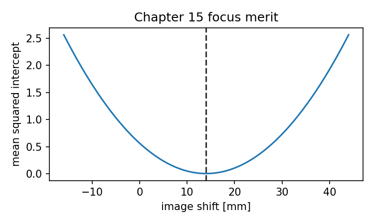
Source and validation note

The least-squares merit function in this chapter is a teaching model. Commercial and research lens-design workflows may use many operand types, constraints, bounds, tolerancing terms, manufacturability penalties, and algorithm choices. The factual claim retained here is narrower: an optimizer follows the explicitly encoded objective and constraints, not an unstated design intention.