Chapter 14: Sampling, Normalization, and the Small Mistakes That Break PSF and MTF

By this point, we have enough code to make convincing plots.

That is good news.

It is also dangerous.

A PSF plot can look smooth and scientific even when the sampling is wrong. An MTF curve can start at 1, fall gracefully, and still have the wrong frequency axis. A Fourier transform can be mathematically valid while representing the wrong physical aperture. A shifted array can produce a result that looks almost right but is centered in the wrong place.

This chapter is a rescue chapter. It adds no new optical concept; it makes the previous three chapters safer.

We have already built this chain:

OPD
→ pupil function
→ PSF
→ OTF
→ MTF

Now we slow down and ask:

When does this chain produce a physically meaningful result?

The answer depends on details that feel small until they break everything:

FFT shift;
array centering;
aperture mask;
zero padding;
pupil sampling;
image-plane sampling;
frequency-axis units;
PSF normalization;
OTF normalization;
wavelength units;
focal length units;
sagittal and tangential directions.

These are not decorative implementation details. They decide what the plot means.

Here is the sharp but useful rule for this chapter:

A correct formula does not save an incorrectly sampled array.

Let us go through the common traps one by one.

1. The problem: beautiful wrong plots

The Fourier transform is extremely obedient.

It does not ask whether your wavelength is in meters or nanometers. It does not know whether your pupil diameter is 5 mm or 5 meters. It does not know whether your zero frequency belongs in the center of the array. It does not know whether your PSF is normalized.

It just transforms the numbers.

That is why FFT-based optics can fail quietly.

A wrong ray-surface intersection often produces an obvious error: rays fly away, intersections disappear, or the code crashes.

A wrong MTF computation may produce a perfectly smooth curve.

This is more dangerous because it looks respectable.

The practical lesson is:

In FFT optics, the first debugging question is not:
“Does the plot look optical?”

It is:
“What are the units, sampling intervals, normalization, and coordinate conventions?”

This chapter gives you a checklist for answering that question.

2. Three arrays, three coordinate systems

The pupil, PSF, and MTF arrays do not live in the same coordinate system.

This is the first source of confusion.

Pupil array

The pupil array describes field across the aperture.

Its coordinates may be:

normalized pupil coordinates

or physical coordinates such as:

meters or millimeters across the pupil

The pupil function is:

$P(x,y)$

where $x,y$ are pupil-plane coordinates.

PSF array

The PSF array describes image-plane intensity.

Its coordinates may be:

angular coordinates

or:

focal-plane length coordinates

The PSF is:

$\mathrm{PSF}(X,Y)$

where $X,Y$ are image-plane coordinates.

MTF array

The MTF array describes spatial frequency response.

Its coordinates are frequency coordinates:

cycles per millimeter

or:

cycles per radian

or sometimes normalized frequency.

The MTF is:

$\mathrm{MTF}(f_x,f_y)$

where $f_x,f_y$ are spatial frequencies.

So the chain is not just:

array → array → array

It is:

pupil-plane field
→ image-plane intensity
→ image-plane spatial-frequency response

That distinction saves a lot of debugging time.

3. The DFT sampling relationship

The discrete Fourier transform connects sampling intervals.

If you sample a function with spacing:

$\Delta x$

and use $N$ samples, the corresponding frequency samples are spaced by:

$\Delta f = \frac{1}{N\Delta x}$

The shifted frequency coordinate is:

$f_k = \frac{k - N/2}{N\Delta x}$

for an even-length array after fftshift.

In NumPy, this is:

freq = np.fft.fftshift(np.fft.fftfreq(N, d=dx))

That one line is the safest way to build a frequency axis.

The important parts are:

N is the number of samples in the transformed array;
dx is the sample spacing in the input domain;
the output unit is cycles per unit of dx.

So if:

dx = 0.01  # millimeters

then:

freq is in cycles per millimeter

If:

dx = 10e-6  # meters

then:

freq is in cycles per meter

The FFT does not attach units. You attach units by using the right dx.

This is the most important sampling idea in the chapter.

4. Pupil sampling to PSF sampling

When we compute a PSF from a pupil function, we are taking a Fourier transform of the pupil field.

For Fraunhofer diffraction, pupil spatial frequency maps to diffraction angle.

A useful practical relationship is:

$\theta = \lambda f_\text{pupil}$

where:

$\theta$ is image angle in radians;
$\lambda$ is wavelength;
$f_\text{pupil}$ is spatial frequency associated with pupil-plane sampling.

If the pupil sample spacing is $\Delta u$ , and the padded pupil array has $N$ samples, then the angular sample spacing is approximately:

$\Delta \theta = \frac{\lambda}{N\Delta u}$

At a focal length $F$ , focal-plane sample spacing is:

$\Delta X = F\Delta\theta$

So:

$\Delta X = \frac{F\lambda}{N\Delta u}$

This formula is worth reading slowly.

It says the PSF sample spacing depends on:

focal length;
wavelength;
padded FFT size;
physical pupil sample spacing.

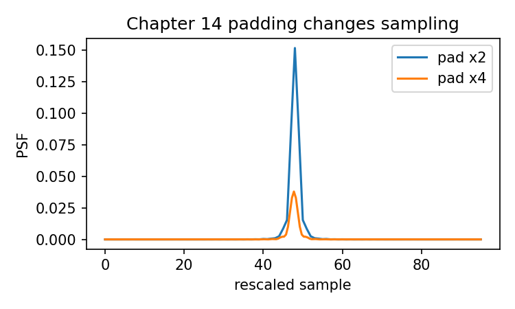
Zero padding changes $N$ , so it changes the displayed PSF sample spacing. It gives more samples in the PSF display.

It does not change the physical aperture.

Here is a helper function:

import numpy as np


def psf_sample_spacing_from_pupil(
    wavelength,
    focal_length,
    pupil_sample_spacing,
    n_fft
):
    """
    Estimate focal-plane PSF sample spacing for Fraunhofer propagation.

    Parameters
    ----------
    wavelength : float
        Wavelength in meters.
    focal_length : float
        Focal length in meters.
    pupil_sample_spacing : float
        Physical spacing between pupil samples, in meters.
    n_fft : int
        FFT array size after padding.

    Returns
    -------
    dx_image : float
        Approximate image-plane sample spacing, in meters.
    """
    dtheta = wavelength / (n_fft * pupil_sample_spacing)
    dx_image = focal_length * dtheta

    return dx_image

If you want the result in millimeters:

dx_image_mm = dx_image * 1e3

This is the bridge from the pupil array to physical PSF coordinates.

5. Example: a physically labeled PSF

Let us create a simple physical setup.

Suppose:

wavelength = 550 nm
focal length = 50 mm
pupil diameter = 10 mm

The f-number is:

$N = \frac{F}{D} = \frac{50}{10} = 5$

Now build the pupil.

import numpy as np
import matplotlib.pyplot as plt


def make_pupil_grid(n=256):
    coord = np.linspace(-1.0, 1.0, n, endpoint=False)
    x, y = np.meshgrid(coord, coord)

    rho = np.sqrt(x**2 + y**2)
    theta = np.arctan2(y, x)
    mask = rho <= 1.0

    return x, y, rho, theta, mask


def pupil_function_from_opd(opd, mask, wavelength, amplitude=None):
    if amplitude is None:
        amplitude = mask.astype(float)

    phase = 2.0 * np.pi * opd / wavelength
    pupil = amplitude * np.exp(1j * phase)
    pupil[~mask] = 0.0 + 0.0j

    return pupil, phase


def pad_array_centered(array, pad_factor=4):
    if pad_factor == 1:
        return array

    n, m = array.shape
    new_n = n * pad_factor
    new_m = m * pad_factor

    padded = np.zeros((new_n, new_m), dtype=array.dtype)

    start_n = (new_n - n) // 2
    start_m = (new_m - m) // 2

    padded[start_n:start_n + n, start_m:start_m + m] = array

    return padded


def compute_psf(pupil, pad_factor=4, normalize=True):
    padded_pupil = pad_array_centered(pupil, pad_factor=pad_factor)

    field = np.fft.fftshift(
        np.fft.fft2(
            np.fft.ifftshift(padded_pupil)
        )
    )

    psf = np.abs(field) ** 2

    if normalize:
        total = np.sum(psf)
        if total > 0:
            psf = psf / total

    return psf, field

Now define the physical parameters:

wavelength = 550e-9      # 550 nm
focal_length = 50e-3     # 50 mm
pupil_diameter = 10e-3   # 10 mm

n_pupil = 256
pad_factor = 4
n_fft = n_pupil * pad_factor

x, y, rho, theta, mask = make_pupil_grid(n=n_pupil)

zero_opd = np.zeros_like(rho)

pupil, _ = pupil_function_from_opd(
    opd=zero_opd,
    mask=mask,
    wavelength=wavelength
)

psf, _ = compute_psf(
    pupil,
    pad_factor=pad_factor
)

The normalized coordinate grid runs from $-1$ to $1$ , representing the full pupil diameter. So a rough pupil sample spacing is:

$\Delta u = \frac{D}{N_\text{pupil}}$

In code:

pupil_sample_spacing = pupil_diameter / n_pupil

dx_image = psf_sample_spacing_from_pupil(
    wavelength=wavelength,
    focal_length=focal_length,
    pupil_sample_spacing=pupil_sample_spacing,
    n_fft=n_fft
)

dx_image_mm = dx_image * 1e3

print("Image-plane sample spacing [mm]:", dx_image_mm)
print("Image-plane sample spacing [um]:", dx_image * 1e6)

Now we can label the PSF axis.

def image_coordinate_axis(n, dx):
    """
    Create centered image-plane coordinate axis.
    """
    center = n // 2
    index = np.arange(n) - center
    return index * dx


coord_image_m = image_coordinate_axis(psf.shape[0], dx_image)
coord_image_um = coord_image_m * 1e6

extent_um = [
    coord_image_um[0],
    coord_image_um[-1],
    coord_image_um[0],
    coord_image_um[-1],
]

plt.figure(figsize=(5, 4))
plt.imshow(psf, origin="lower", extent=extent_um)
plt.colorbar(label="Normalized intensity")
plt.xlabel("Image x [um]")
plt.ylabel("Image y [um]")
plt.title("Diffraction-limited PSF with physical axis")
plt.tight_layout()
plt.show()

Now the PSF plot is not just an array image. Its axis has a physical interpretation.

This is a big improvement.

But it also creates responsibility. If the pupil diameter, focal length, wavelength, or padding size is wrong, the axis label is wrong.

6. Checking the Airy radius

A good sanity check is the Airy first dark ring.

For a circular aperture, the first dark ring radius in the focal plane is approximately:

$r_\text{Airy} = 1.22\lambda N$

where $N$ is the f-number.

With:

λ = 550 nm
N = 5

we get:

$r_\text{Airy} = 1.22 \times 550\text{ nm} \times 5$

$r_\text{Airy} \approx 3.36\ \mu\text{m}$

Code:

f_number = focal_length / pupil_diameter
airy_radius = 1.22 * wavelength * f_number

print("F-number:", f_number)
print("Airy first dark radius [um]:", airy_radius * 1e6)

This gives us a rough check on the PSF axis.

The first dark ring in the plotted PSF should be near that radius.

It may not match perfectly because of sampling, finite array effects, display interpolation, and how we locate the minimum. But if the ring appears at 3 meters or 0.003 nanometers, something is wrong.

This kind of sanity check is not optional in computational optics.

A good habit is:

After computing a diffraction-limited PSF,
check whether the Airy scale is physically plausible.

This one check catches many unit mistakes.

7. Wrong sampling example: the same PSF with the wrong pupil diameter

Let us intentionally make a mistake.

Suppose the actual pupil diameter is 10 mm, but we accidentally label it as 1 mm.

The computed PSF array does not change. Why? Because the array values came from the normalized pupil mask.

But the physical axis changes dramatically.

wrong_pupil_diameter = 1e-3  # wrong: 1 mm instead of 10 mm

wrong_pupil_sample_spacing = wrong_pupil_diameter / n_pupil

wrong_dx_image = psf_sample_spacing_from_pupil(
    wavelength=wavelength,
    focal_length=focal_length,
    pupil_sample_spacing=wrong_pupil_sample_spacing,
    n_fft=n_fft
)

print("Correct dx [um]:", dx_image * 1e6)
print("Wrong dx [um]:", wrong_dx_image * 1e6)

Because the pupil sample spacing became ten times smaller, the image-plane sample spacing becomes ten times larger.

The PSF image still looks like an Airy pattern. But its physical size is mislabeled.

This is the quiet failure mode.

The numerical array is not enough. The coordinate model matters.

The wrong plot may look optical. It may even look beautiful. But it describes a different physical system.

8. From PSF sampling to MTF frequency axis

Now we move one step forward.

The MTF is computed from the PSF. Its frequency axis is determined by the PSF sample spacing.

If the PSF sample spacing is $\Delta X$ , the MTF frequency samples are:

$f_k = \frac{k - N/2}{N\Delta X}$

In NumPy:

freq = np.fft.fftshift(np.fft.fftfreq(N, d=dx_image))

If dx_image is in meters, freq is in cycles per meter.

For cycles per millimeter:

freq_cyc_per_mm = freq / 1000.0

because one meter contains 1000 millimeters, and cycles/m divided by 1000 gives cycles/mm.

Here is a clean MTF computation with axis generation:

def compute_otf_mtf(psf):
    otf = np.fft.fftshift(
        np.fft.fft2(
            np.fft.ifftshift(psf)
        )
    )

    center = (otf.shape[0] // 2, otf.shape[1] // 2)

    if np.abs(otf[center]) > 0:
        otf = otf / otf[center]

    mtf = np.abs(otf)

    return otf, mtf


def mtf_frequency_axis(n, dx_image):
    """
    Frequency axis for MTF.

    Parameters
    ----------
    n : int
        Number of PSF / MTF samples.
    dx_image : float
        PSF sample spacing in meters.

    Returns
    -------
    freq_cyc_per_mm : 1D array
        Spatial frequency in cycles/mm.
    """
    freq_cyc_per_m = np.fft.fftshift(
        np.fft.fftfreq(n, d=dx_image)
    )

    freq_cyc_per_mm = freq_cyc_per_m / 1000.0

    return freq_cyc_per_mm

Now compute and plot:

otf, mtf = compute_otf_mtf(psf)

freq = mtf_frequency_axis(
    n=mtf.shape[0],
    dx_image=dx_image
)

center = mtf.shape[0] // 2
mtf_slice = mtf[center, :]

plt.figure(figsize=(6, 4))
plt.plot(freq[center:], mtf_slice[center:])
plt.xlabel("Spatial frequency [cycles/mm]")
plt.ylabel("MTF")
plt.ylim(0, 1.05)
plt.title("Diffraction-limited MTF")
plt.grid(True)
plt.tight_layout()
plt.show()

Now the x-axis has a physical meaning.

9. Checking the diffraction cutoff

For incoherent diffraction-limited imaging with a circular aperture, the cutoff frequency is approximately:

$f_c = \frac{1}{\lambda N}$

where:

$f_c$ is in cycles per length;
$\lambda$ uses the same length unit;
$N$ is the f-number.

If $\lambda$ is in millimeters, $f_c$ is cycles/mm.

wavelength_mm = wavelength * 1e3
cutoff_cyc_per_mm = 1.0 / (wavelength_mm * f_number)

print("Diffraction cutoff [cycles/mm]:", cutoff_cyc_per_mm)

For 550 nm and f/5, the cutoff is approximately:

$f_c \approx 364\ \text{cycles/mm}$

The MTF should approach zero around that frequency.

Again, it will not be perfect in a small teaching script. But it should be in the right neighborhood.

If your plotted MTF goes to zero at 3.64 cycles/mm or 3,640,000 cycles/mm, suspect a unit error.

The cutoff gives a strong sanity check:

Airy radius checks the PSF axis.
Diffraction cutoff checks the MTF axis.

These two checks should become automatic.

10. Wrong MTF axis example

Let us intentionally make the MTF axis wrong by using the wrong PSF sample spacing.

The MTF values are the same, but the frequency labels change.

wrong_freq = mtf_frequency_axis(
    n=mtf.shape[0],
    dx_image=wrong_dx_image
)

plt.figure(figsize=(7, 4))
plt.plot(freq[center:], mtf_slice[center:], label="Correct axis")
plt.plot(wrong_freq[center:], mtf_slice[center:], "--", label="Wrong axis")
plt.xlabel("Spatial frequency [cycles/mm]")
plt.ylabel("MTF")
plt.ylim(0, 1.05)
plt.title("Same MTF values, different frequency labels")
plt.grid(True)
plt.legend()
plt.tight_layout()
plt.show()

This is the exact kind of error that can survive visual inspection.

The curve shape is identical. Only the x-axis changes.

But for engineering interpretation, that is not a small problem. It changes the answer to questions like:

What is the MTF at 50 cycles/mm?
What is the cutoff frequency?
How does this compare with a sensor pixel pitch?

A mislabeled frequency axis can turn a weak system into a strong one, or a strong one into a weak one.

The curve shape alone is not enough.

11. FFT shift: where is the center?

FFT shift errors are another classic trap.

NumPy’s FFT functions use an array convention where zero frequency is at the beginning of the array before shifting.

For display and optical interpretation, we often want zero frequency or the PSF peak at the center.

So we use:

np.fft.fftshift(...)

and sometimes:

np.fft.ifftshift(...)

The common pattern for PSF from pupil is:

field = np.fft.fftshift(
    np.fft.fft2(
        np.fft.ifftshift(pupil)
    )
)

The common pattern for OTF from PSF is:

otf = np.fft.fftshift(
    np.fft.fft2(
        np.fft.ifftshift(psf)
    )
)

Keep centered arrays centered through the transform.

There are several valid conventions, but mixing conventions is dangerous.

A practical test:

peak_index = np.unravel_index(np.argmax(psf), psf.shape)
print("PSF peak index:", peak_index)
print("Expected center:", (psf.shape[0] // 2, psf.shape[1] // 2))

For an on-axis perfect pupil, the PSF peak should be at or very near the center.

If it appears in a corner, your shift convention is wrong for your display.

For the MTF:

otf_center = (otf.shape[0] // 2, otf.shape[1] // 2)
print("OTF center value:", otf[otf_center])
print("MTF center value:", mtf[otf_center])

The MTF center should be close to 1 after normalization.

These checks are simple. Use them.

12. Odd and even array sizes

Even-sized and odd-sized arrays have slightly different center behavior.

For an even array with $N=1024$ , the center index after fftshift is:

N // 2

For an odd array with $N=1025$ , it is also:

N // 2

but the symmetry around the center is slightly different.

This does not mean odd sizes are forbidden. It means you should be consistent and test where the peak and zero frequency appear.

For teaching code, powers of two or even sizes are convenient:

256, 512, 1024

They are not required by modern FFT libraries, but they make examples clean.

When debugging, avoid changing too many things at once. Do not simultaneously change:

array size;
padding factor;
aperture diameter;
wavelength;
FFT shift convention.

Change one thing and observe what happens.

That is slow, but it works.

13. Zero padding: interpolation, not extra physics

Zero padding is useful, but it is often misunderstood.

When you zero-pad the pupil before computing the PSF, you increase the number of samples in the Fourier-domain output.

The displayed PSF becomes smoother.

But the physical aperture has not changed. The optical resolution has not improved.

The correct statement is:

Zero padding interpolates the sampled PSF.
It does not create new optical information.

Let us compare padding factors.

pad_factors = [1, 2, 4, 8]

plt.figure(figsize=(7, 4))

for pf in pad_factors:
    psf_pf, _ = compute_psf(pupil, pad_factor=pf)

    n_fft_pf = n_pupil * pf
    dx_pf = psf_sample_spacing_from_pupil(
        wavelength=wavelength,
        focal_length=focal_length,
        pupil_sample_spacing=pupil_sample_spacing,
        n_fft=n_fft_pf
    )

    axis_pf = image_coordinate_axis(psf_pf.shape[0], dx_pf) * 1e6
    center_pf = psf_pf.shape[0] // 2
    slice_pf = psf_pf[center_pf, :]

    plt.plot(axis_pf, slice_pf / np.max(slice_pf), label=f"pad {pf}")

plt.xlim(-15, 15)
plt.xlabel("Image coordinate [um]")
plt.ylabel("Normalized peak intensity")
plt.title("Zero padding changes display sampling")
plt.grid(True)
plt.legend()
plt.tight_layout()
plt.show()

The curves should describe the same diffraction pattern, but higher padding gives a smoother sampled profile.

If padding changes the physical interpretation dramatically, something else is wrong.

A useful check is:

The Airy radius should not change when padding changes.
The number of samples across it should change.

That sentence is a good debugging tool.

14. PSF normalization: peak or energy?

There are two common normalizations for PSF display.

Energy normalization

Total PSF sum equals 1:

$\sum \mathrm{PSF} = 1$

Code:

psf_energy = psf / np.sum(psf)

This is useful when comparing energy distribution.

Peak normalization

Peak PSF value equals 1:

$\max(\mathrm{PSF}) = 1$

Code:

psf_peak = psf / np.max(psf)

This is useful for plotting profiles or comparing shapes visually.

They answer different questions.

Energy normalization preserves total energy comparison. Peak normalization makes central peaks visually comparable.

For Strehl ratio, you need matching energy normalization and sampling:

strehl = np.max(aberrated_psf_energy) / np.max(perfect_psf_energy)

If one PSF is peak-normalized and the other is energy-normalized, the ratio is meaningless.

This is one of those mistakes that can sit quietly inside a notebook.

A practical habit:

Name normalized arrays clearly:
psf_energy_normalized
psf_peak_normalized

Do not call everything psf.

15. OTF normalization: divide by the DC value

The OTF is the Fourier transform of the PSF.

The zero-frequency value of the OTF is the total energy of the PSF. If the PSF sum is 1, the OTF center should be 1 after shifting.

But numerical scaling and normalization choices can still vary.

So we usually normalize:

center = (otf.shape[0] // 2, otf.shape[1] // 2)
otf = otf / otf[center]
mtf = np.abs(otf)

This makes:

MTF at zero frequency = 1

A basic check:

print(mtf[center])

It should be very close to:

1.0

If it is not, check:

PSF centering;
OTF shift;
OTF center index;
PSF normalization;
accidental complex or negative PSF values.

The zero-frequency point is your anchor. Do not ignore it.

16. Wrong normalization example

Let us create two PSFs: perfect and aberrated.

def synthetic_opd(rho, theta, mask, wavelength):
    opd = np.zeros_like(rho)

    defocus = 0.50 * wavelength
    astigmatism = 0.25 * wavelength

    opd += defocus * (2.0 * rho**2 - 1.0)
    opd += astigmatism * rho**2 * np.cos(2.0 * theta)

    opd[~mask] = 0.0

    return opd


aberrated_opd = synthetic_opd(
    rho=rho,
    theta=theta,
    mask=mask,
    wavelength=wavelength
)

aberrated_pupil, _ = pupil_function_from_opd(
    opd=aberrated_opd,
    mask=mask,
    wavelength=wavelength
)

perfect_psf, _ = compute_psf(
    pupil,
    pad_factor=4,
    normalize=True
)

aberrated_psf, _ = compute_psf(
    aberrated_pupil,
    pad_factor=4,
    normalize=True
)

Now compute Strehl correctly:

strehl_correct = np.max(aberrated_psf) / np.max(perfect_psf)
print("Correct Strehl:", strehl_correct)

Now make a bad comparison by peak-normalizing both first:

perfect_peak_norm = perfect_psf / np.max(perfect_psf)
aberrated_peak_norm = aberrated_psf / np.max(aberrated_psf)

strehl_wrong = np.max(aberrated_peak_norm) / np.max(perfect_peak_norm)
print("Wrong Strehl after peak normalization:", strehl_wrong)

The wrong result will be 1.

That is obviously useless. We erased the peak difference before calculating the peak ratio.

This example is simple, but the lesson is general:

Normalize after deciding what quantity you are trying to compare.

Not before.

17. Aperture mask: the square-array trap

A square NumPy array is not a circular aperture.

This mistake is easy to make:

pupil_wrong = np.ones((256, 256), dtype=complex)

This does not represent a clear circular lens aperture. It represents a square aperture.

A square aperture has a different diffraction pattern and a different MTF.

The correct circular pupil needs a mask:

pupil_correct = mask.astype(complex)

Let us compare:

square_pupil = np.ones_like(pupil, dtype=complex)

square_psf, _ = compute_psf(square_pupil, pad_factor=4)
circular_psf, _ = compute_psf(pupil, pad_factor=4)

square_otf, square_mtf = compute_otf_mtf(square_psf)
circular_otf, circular_mtf = compute_otf_mtf(circular_psf)

center = circular_mtf.shape[0] // 2
freq = mtf_frequency_axis(circular_mtf.shape[0], dx_image)

plt.figure(figsize=(7, 4))
plt.plot(freq[center:], circular_mtf[center, center:], label="Circular pupil")
plt.plot(freq[center:], square_mtf[center, center:], "--", label="Square pupil")
plt.xlabel("Spatial frequency [cycles/mm]")
plt.ylabel("MTF")
plt.ylim(0, 1.05)
plt.title("Aperture shape changes MTF")
plt.grid(True)
plt.legend()
plt.tight_layout()
plt.show()

The difference is not a numerical accident. It is physics.

Aperture shape affects diffraction.

So the first check before computing PSF is:

Does the pupil array represent the aperture I think it represents?

Plot the pupil amplitude before Fourier-transforming it.

Always.

18. Endpoint sampling: `linspace` can quietly change your grid

In earlier chapters, we often used:

coord = np.linspace(-1.0, 1.0, n)

This includes both endpoints by default.

For many teaching plots, this is acceptable. But for FFT sampling, including both $-1$ and $1$ can be slightly awkward because those endpoints represent duplicate edges of a periodic sampling interval.

A more FFT-friendly version is:

coord = np.linspace(-1.0, 1.0, n, endpoint=False)

This samples the interval without duplicating the endpoint.

Will this destroy your result if you use the default? Usually not in a beginner example. But it can create small asymmetries and sampling differences.

For careful FFT work, prefer explicit sampling:

coord = (np.arange(n) - n / 2) / (n / 2)

or:

coord = np.linspace(-1.0, 1.0, n, endpoint=False)

The deeper rule is:

Know whether your grid includes the endpoint.
Do not let default sampling choices define your optical model silently.

This is one reason production optical software has careful internal sampling conventions.

19. Units: the most boring and most powerful debugging tool

Units are not clerical decoration.

They are part of the computation.

Here are the most common unit pairings in this part of the book:

OPD: meters
wavelength: meters
phase: radians

pupil diameter: meters
focal length: meters
PSF coordinate: meters

PSF sample spacing: millimeters
MTF frequency: cycles/mm

The dangerous case is mixed hidden units:

wavelength = 550       # meant nanometers
focal_length = 50      # meant millimeters
pupil_diameter = 10    # meant millimeters

This code may run, but it has no reliable physical meaning.

A safer style is:

wavelength = 550e-9
focal_length = 50e-3
pupil_diameter = 10e-3

Then convert only for display:

print(dx_image * 1e6, "um")
print(freq / 1000.0, "cycles/mm")

A simple discipline helps:

Use SI units inside the computation.
Convert units only at input and output boundaries.

That one habit prevents many mistakes.

20. Sign conventions and mirrored results

In Chapter 11, we mentioned that pupil phase sign conventions can differ:

$P(x,y)=A(x,y)\exp\left(i\frac{2\pi W(x,y)}{\lambda}\right)$

or:

$P(x,y)=A(x,y)\exp\left(-i\frac{2\pi W(x,y)}{\lambda}\right)$

Changing the sign may mirror or conjugate parts of the field behavior depending on the aberration and Fourier convention.

For symmetric aberrations, the intensity PSF may look similar. For asymmetric aberrations, such as coma-like phase, the PSF can flip direction.

This means two implementations may disagree visually while both are internally consistent.

A practical comparison checklist:

same OPD definition
same phase sign
same pupil coordinate orientation
same FFT convention
same display orientation

Do not compare only the final plot. Compare intermediate arrays:

OPD map;
phase map;
pupil amplitude;
pupil phase;
PSF center;
MTF center value.

When a final PSF appears mirrored, the error may be in a sign convention or coordinate orientation, not in diffraction theory.

21. Sagittal and tangential directions: do not guess

For on-axis systems with rotational symmetry, horizontal and vertical MTF slices may be nearly identical.

For off-axis fields, sagittal and tangential directions matter.

But they are not simply “x” and “y” in every plot.

They are defined relative to:

the optical axis;
the field point;
the chief ray or meridional plane.

So this is careless:

horizontal = tangential
vertical = sagittal

It may be true in a particular coordinate setup. It is not universally true.

A safer teaching statement is:

Horizontal and vertical slices are array directions.
Sagittal and tangential slices are optical field directions.

To compare with Optiland or any optical design software, check how the software defines these directions for the selected field.

A good debugging question is:

Which direction in my array corresponds to the field's tangential plane?

Without that answer, labels such as sagittal and tangential are decorative, not trustworthy.

22. A small diagnostic toolkit

Now let us collect a few functions that make debugging easier.

These are not fancy. They are practical.

def check_array_center(name, array):
    """
    Print the peak location of a real-valued array.
    Useful for PSF and MTF checks.
    """
    peak = np.unravel_index(np.argmax(np.abs(array)), array.shape)
    center = (array.shape[0] // 2, array.shape[1] // 2)

    print(f"{name}")
    print("  shape: ", array.shape)
    print("  peak:  ", peak)
    print("  center:", center)
    print()


def check_psf_normalization(psf):
    """
    Print basic PSF normalization information.
    """
    print("PSF checks")
    print("  sum: ", np.sum(psf))
    print("  max: ", np.max(psf))
    print("  min: ", np.min(psf))
    print()


def check_mtf_normalization(mtf):
    """
    Print MTF center value.
    """
    center = (mtf.shape[0] // 2, mtf.shape[1] // 2)

    print("MTF checks")
    print("  center value:", mtf[center])
    print("  max value:   ", np.max(mtf))
    print("  min value:   ", np.min(mtf))
    print()

Use them:

check_array_center("PSF", psf)
check_psf_normalization(psf)

otf, mtf = compute_otf_mtf(psf)
check_array_center("MTF", mtf)
check_mtf_normalization(mtf)

For a centered, diffraction-limited PSF:

PSF peak should be near the center;
PSF sum should be 1 if energy-normalized;
MTF center should be 1;
MTF maximum should usually be close to 1.

These checks do not prove everything is correct. But they catch common failures quickly.

23. A full corrected PSF/MTF workflow

Here is a compact workflow that keeps the bookkeeping explicit.

import numpy as np
import matplotlib.pyplot as plt


def make_pupil_grid(n=256):
    coord = np.linspace(-1.0, 1.0, n, endpoint=False)
    x, y = np.meshgrid(coord, coord)

    rho = np.sqrt(x**2 + y**2)
    theta = np.arctan2(y, x)
    mask = rho <= 1.0

    return x, y, rho, theta, mask


def pupil_function_from_opd(opd, mask, wavelength, amplitude=None):
    if amplitude is None:
        amplitude = mask.astype(float)

    phase = 2.0 * np.pi * opd / wavelength
    pupil = amplitude * np.exp(1j * phase)
    pupil[~mask] = 0.0 + 0.0j

    return pupil, phase


def pad_array_centered(array, pad_factor=4):
    if pad_factor == 1:
        return array

    n, m = array.shape
    new_n = n * pad_factor
    new_m = m * pad_factor

    padded = np.zeros((new_n, new_m), dtype=array.dtype)

    start_n = (new_n - n) // 2
    start_m = (new_m - m) // 2

    padded[start_n:start_n + n, start_m:start_m + m] = array

    return padded


def compute_psf(pupil, pad_factor=4):
    padded_pupil = pad_array_centered(pupil, pad_factor=pad_factor)

    field = np.fft.fftshift(
        np.fft.fft2(
            np.fft.ifftshift(padded_pupil)
        )
    )

    psf = np.abs(field) ** 2
    psf = psf / np.sum(psf)

    return psf, field


def compute_otf_mtf(psf):
    otf = np.fft.fftshift(
        np.fft.fft2(
            np.fft.ifftshift(psf)
        )
    )

    center = (otf.shape[0] // 2, otf.shape[1] // 2)
    otf = otf / otf[center]

    mtf = np.abs(otf)

    return otf, mtf


def psf_sample_spacing_from_pupil(
    wavelength,
    focal_length,
    pupil_sample_spacing,
    n_fft
):
    dtheta = wavelength / (n_fft * pupil_sample_spacing)
    return focal_length * dtheta


def image_coordinate_axis(n, dx):
    center = n // 2
    return (np.arange(n) - center) * dx


def mtf_frequency_axis(n, dx_image):
    freq_cyc_per_m = np.fft.fftshift(
        np.fft.fftfreq(n, d=dx_image)
    )
    return freq_cyc_per_m / 1000.0


# Physical parameters, SI units inside the computation
wavelength = 550e-9
focal_length = 50e-3
pupil_diameter = 10e-3

# Sampling parameters
n_pupil = 256
pad_factor = 4
n_fft = n_pupil * pad_factor

# Build pupil
x, y, rho, theta, mask = make_pupil_grid(n=n_pupil)
opd = np.zeros_like(rho)

pupil, phase = pupil_function_from_opd(
    opd=opd,
    mask=mask,
    wavelength=wavelength
)

# Compute PSF
psf, field = compute_psf(
    pupil=pupil,
    pad_factor=pad_factor
)

# Coordinate bookkeeping
pupil_sample_spacing = pupil_diameter / n_pupil

dx_image = psf_sample_spacing_from_pupil(
    wavelength=wavelength,
    focal_length=focal_length,
    pupil_sample_spacing=pupil_sample_spacing,
    n_fft=n_fft
)

image_axis_um = image_coordinate_axis(psf.shape[0], dx_image) * 1e6

# Compute MTF
otf, mtf = compute_otf_mtf(psf)
freq_cyc_per_mm = mtf_frequency_axis(mtf.shape[0], dx_image)

# Sanity checks
f_number = focal_length / pupil_diameter
airy_radius_um = 1.22 * wavelength * f_number * 1e6
cutoff_cyc_per_mm = 1.0 / ((wavelength * 1e3) * f_number)

print("F-number:", f_number)
print("Airy first dark radius [um]:", airy_radius_um)
print("PSF sample spacing [um]:", dx_image * 1e6)
print("Diffraction cutoff [cycles/mm]:", cutoff_cyc_per_mm)

# Plot PSF
extent_um = [
    image_axis_um[0],
    image_axis_um[-1],
    image_axis_um[0],
    image_axis_um[-1],
]

plt.figure(figsize=(5, 4))
plt.imshow(psf, origin="lower", extent=extent_um)
plt.colorbar(label="Normalized intensity")
plt.xlabel("Image x [um]")
plt.ylabel("Image y [um]")
plt.title("PSF with physical coordinates")
plt.tight_layout()
plt.show()

# Plot MTF slice
center = mtf.shape[0] // 2

plt.figure(figsize=(6, 4))
plt.plot(freq_cyc_per_mm[center:], mtf[center, center:])
plt.xlabel("Spatial frequency [cycles/mm]")
plt.ylabel("MTF")
plt.ylim(0, 1.05)
plt.title("MTF with physical frequency axis")
plt.grid(True)
plt.tight_layout()
plt.show()

This is not the shortest possible code.

That is intentional.

This version favors traceability over compactness.

Each physical parameter is visible. Each sampling step is explicit. Each output axis is derived from known quantities.

This is the kind of code that is easier to trust.

24. Optiland comparison: what to check before blaming the library

When comparing this teaching code with Optiland, do not expect a match by accident.

A real optical design library may include more careful handling of:

exit pupil geometry;
reference sphere;
field-dependent pupil mapping;
wavelength weighting;
image-space refractive index;
focus position;
vignetting;
polarization;
sampling strategies;
internal normalization;
sagittal/tangential definitions.

So a mismatch is not automatically a bug.

Before blaming the library or your code, check:

1. Same optical system?
2. Same field point?
3. Same wavelength?
4. Same aperture stop and pupil diameter?
5. Same focus plane?
6. Same OPD reference?
7. Same pupil sampling?
8. Same FFT padding?
9. Same PSF normalization?
10. Same MTF frequency units?
11. Same sagittal/tangential definitions?
12. Same display scale?

A validation-style comparison workflow looks like this:

# Version-checked workflow outline.
# Check your installed Optiland version for exact API names.

# 1. Build or load the optical system.
# optic = ...

# 2. Set wavelength, field point, aperture, and focus.
# wavelength = ...
# field = ...

# 3. Generate PSF and MTF with Optiland analysis tools.
# psf_optiland = ...
# mtf_optiland = ...

# 4. Extract or reconstruct comparable arrays if available.
# psf_array = ...
# dx_image = ...

# 5. Recompute OTF/MTF from the sampled PSF.
# otf_numpy, mtf_numpy = compute_otf_mtf(psf_array)

# 6. Compare:
# - PSF peak location
# - PSF sum
# - MTF at zero frequency
# - frequency axis
# - cutoff frequency
# - sagittal/tangential direction definitions

The educational purpose is not to prove that your tiny script is more correct than Optiland. It is not.

The purpose is to understand what must be aligned before two calculations can be compared.

This is a very practical form of understanding.

25. Debugging sequence for a suspicious PSF

When a PSF looks wrong, do not randomly change code.

Use a sequence.

Step 1: Check the pupil amplitude

Plot:

plt.imshow(np.abs(pupil), origin="lower")
plt.colorbar(label="Amplitude")
plt.title("Pupil amplitude")
plt.show()

Ask:

Is the aperture shape correct?
Is the central obstruction included or excluded as intended?
Is anything outside the aperture nonzero?

Step 2: Check the pupil phase

Plot:

plt.imshow(np.angle(pupil), origin="lower")
plt.colorbar(label="Phase [rad]")
plt.title("Wrapped pupil phase")
plt.show()

Ask:

Does the phase pattern match the expected OPD?
Are phase wraps expected?
Are units consistent?

Step 3: Check PSF centering

check_array_center("PSF", psf)

Ask:

Is the peak near the center for an on-axis point?

Step 4: Check PSF energy

check_psf_normalization(psf)

Ask:

Does the PSF sum equal 1 after normalization?

Step 5: Check physical scale

Compute:

airy_radius = 1.22 * wavelength * f_number

Ask:

Is the Airy scale plausible?

That sequence catches most beginner errors.

26. Debugging sequence for a suspicious MTF

When an MTF curve looks wrong, use a different sequence.

Step 1: Check PSF first

Do not debug MTF before checking PSF.

A wrong PSF cannot produce a right MTF.

Step 2: Check OTF center

center = (otf.shape[0] // 2, otf.shape[1] // 2)
print(otf[center])

After normalization, the center should be close to:

1 + 0j

Step 3: Check MTF center

print(mtf[center])

It should be close to:

Step 4: Check frequency axis

Compute the diffraction cutoff:

cutoff_cyc_per_mm = 1.0 / ((wavelength * 1e3) * f_number)

Ask:

Does the MTF approach zero near the expected cutoff?

Step 5: Check direction labels

Ask:

Are these array slices, or true sagittal/tangential slices?

Step 6: Check display range

Make sure the plot is not hiding negative, clipped, or out-of-range values.

For MTF:

plt.ylim(0, 1.05)

is often useful for a first check.

27. The most common failure patterns

Here is a compact table of symptoms and likely causes.

Symptom	Likely cause
PSF peak appears in a corner	Missing or inconsistent `fftshift` / `ifftshift`
PSF looks like a square-aperture diffraction pattern	Forgot circular aperture mask
PSF physical size is wildly wrong	Wrong pupil diameter, focal length, wavelength, or padding in coordinate calculation
MTF does not start at 1	OTF not normalized by DC value, wrong center index, or PSF issue
MTF cutoff is far from expected value	Wrong PSF sample spacing or unit conversion
Strehl ratio becomes 1 for every case	PSFs were peak-normalized before computing Strehl
Sagittal and tangential labels disagree with software	Direction definitions do not match field geometry
Log PSF looks dramatic but linear PSF looks fine	Display scale difference, not necessarily physical disaster
Changing padding appears to change optical resolution	Misinterpreting zero padding or axis scaling
Aberrated PSF is mirrored compared with reference	Sign convention or coordinate orientation mismatch

This table is not a substitute for understanding. It is a triage tool.

When something breaks, it gives you the first places to look.

28. Why this chapter belongs before optimization

It may feel tempting to move straight from MTF to optimization.

After all, once we can compute MTF, why not start improving it?

Because optimization amplifies mistakes.

If the PSF is mis-scaled, an optimizer can improve the wrong metric.

If the MTF frequency axis is wrong, an optimizer can favor the wrong spatial frequencies.

If normalization is inconsistent, an optimizer can appear to improve performance by changing energy scale rather than image quality.

If sagittal and tangential directions are mislabeled, an optimizer can fix the wrong directional behavior.

Optimization does not make a bad metric honest.

It only follows the metric you give it.

That is why this chapter sits here.

Before we ask software to improve a lens, we need to know what our numbers mean.

The chain should now be read with safeguards:

pupil function
→ checked amplitude and phase
→ PSF with known sampling and normalization
→ OTF normalized at DC
→ MTF with correct frequency axis and direction labels

Only then is it reasonable to use these quantities inside a merit function.

29. The practical checklist

Use this checklist whenever you compute PSF or MTF.

Pupil checks

[ ] Is the aperture mask correct?
[ ] Is amplitude field amplitude, not intensity?
[ ] Is OPD in the same length unit as wavelength?
[ ] Is the phase sign convention known?
[ ] Is the pupil coordinate orientation known?
[ ] Is the pupil sampled densely enough?

PSF checks

[ ] Is the FFT shift convention consistent?
[ ] Is the PSF peak centered for an on-axis point?
[ ] Is the PSF energy normalized when needed?
[ ] Is zero padding interpreted as interpolation, not better optics?
[ ] Is the PSF axis derived from pupil sampling, wavelength, and focal length?
[ ] Does the Airy radius look plausible for a perfect circular pupil?

MTF checks

[ ] Is OTF computed from PSF, not directly from OPD or pupil?
[ ] Is OTF normalized by its zero-frequency value?
[ ] Does MTF start at 1?
[ ] Is the frequency axis in the intended unit?
[ ] Does the diffraction cutoff look plausible?
[ ] Are sagittal and tangential directions defined correctly?

Comparison checks

[ ] Same wavelength?
[ ] Same field point?
[ ] Same focus plane?
[ ] Same aperture and pupil definition?
[ ] Same sampling density?
[ ] Same normalization?
[ ] Same display scale?
[ ] Same coordinate orientation?

This checklist may look plain. In real work, plain checklists save hours.

30. What this chapter adds to the full chain

The previous chapters gave us the formulas:

$P(x,y)=A(x,y)\exp\left(i\frac{2\pi W(x,y)}{\lambda}\right)$

$\mathrm{PSF}=|\mathcal{F}{P(x,y)}|^2$

$\mathrm{OTF}=\mathcal{F}{\mathrm{PSF}}$

$\mathrm{MTF}=|\mathrm{OTF}|$

This chapter adds the conditions that make those formulas meaningful in code.

It tells us that every transform needs sampling, every plot needs units, and every comparison needs normalization.

So the real computational chain is not only:

OPD
→ pupil
→ PSF
→ MTF

It is closer to:

OPD with correct units
→ pupil with correct mask and phase convention
→ PSF with correct FFT shift, sampling, and normalization
→ OTF normalized at zero frequency
→ MTF with correct frequency axis and direction labels

That longer version is less elegant.

It is also closer to the truth.

The next chapter moves into optimization. We will finally ask what optical software is doing when it “improves” a design.

But now we can ask that question safely.

Optimization is not magic. It is repeated calculation guided by a merit function.

And after this chapter, we know something important:

Before optimizing an optical metric, make sure the metric means what you think it means.

Chapter summary

FFT-based PSF and MTF calculations are powerful, but they are sensitive to sampling, units, centering, and normalization.

The DFT sampling relationship is:

$\Delta f = \frac{1}{N\Delta x}$

For PSF calculation from a physical pupil, the approximate focal-plane sample spacing is:

$\Delta X = \frac{F\lambda}{N\Delta u}$

where $F$ is focal length, $\lambda$ is wavelength, $N$ is the padded FFT size, and $\Delta u$ is pupil-plane sample spacing.

For MTF, the frequency axis comes from the PSF sample spacing:

freq = np.fft.fftshift(np.fft.fftfreq(n, d=dx_image))

The PSF should be checked against the Airy radius:

$r_\text{Airy}=1.22\lambda N$

and the MTF should be checked against the diffraction cutoff:

$f_c=\frac{1}{\lambda N}$

where $N$ is the f-number.

Zero padding improves display sampling but does not improve physical optical resolution. PSF energy normalization, PSF peak normalization, and OTF DC normalization serve different purposes and should not be mixed casually.

The most important practical habit is to inspect intermediate results:

pupil amplitude
pupil phase
PSF center and energy
OTF center value
MTF frequency axis

A plot is only trustworthy when its sampling and units are trustworthy.

Generated validation figure

Padding and sampling comparison generated from the Chapter 14 sampling check

Keyboard shortcuts

Computational Optics