Chapter 13: OTF and MTF: Turning a PSF into a Frequency Response

We began this book with a curve.

An MTF curve appears in optical design software as if it were a finished verdict: sharp here, weak there, better in one field, worse in another. It looks clean. It looks authoritative. It is easy to read just enough of it to become dangerous.

But an MTF curve is not born as a curve.

It is the end of a calculation chain.

By now, that chain is no longer hidden:

lens prescription
→ ray tracing
→ optical path length
→ OPD
→ pupil function
→ PSF
→ OTF
→ MTF

In Chapter 12, we computed the PSF from the complex pupil function. The PSF told us how one ideal point spreads out in the image plane.

Now we ask a different question:

If the object contains patterns of different spatial frequencies,
how strongly does the optical system transfer each one?

That question leads to the optical transfer function, or OTF.

The MTF, or modulation transfer function, is the magnitude of the OTF.

In minimal form:

$$\mathrm{OTF} = \mathcal{F}{\mathrm{PSF}}$$

$$\mathrm{MTF} = |\mathrm{OTF}|$$

Those two lines are simple. Their meaning is not small.

This chapter is where the PSF stops being only an image of a point and becomes a frequency response.

1. Why MTF exists at all

The PSF answers:

What does the system do to one point?

MTF answers:

What does the system do to contrast at different detail sizes?

An object can be thought of as containing many spatial frequencies.

Large, slow changes are low spatial frequencies. Fine details are high spatial frequencies.

For example:

• a broad gray patch is low frequency;
• a thick black-white stripe pattern is lower frequency;
• a very fine stripe pattern is higher frequency;
• tiny texture, hair, fabric weave, or fine printed text contains high frequencies.

An optical system does not transmit all these frequencies equally.

Low-frequency contrast may survive well. High-frequency contrast may be weakened. At some point, fine detail may no longer be transferred with useful contrast.

That is what the MTF curve shows.

A typical MTF curve begins near 1 at zero frequency and drops as frequency increases.

This does not mean every system drops smoothly in every direction. Real systems can have structure, directional differences, field dependence, wavelength dependence, and sampling issues. But the first mental model is:

MTF tells us how contrast transfer changes with spatial frequency.

That sentence is useful. It is also incomplete. The rest of the chapter makes it computable.

2. PSF as an impulse response

To understand why the Fourier transform of the PSF gives the OTF, we need one idea from imaging theory.

For an incoherent, shift-invariant imaging system, the image can be modeled as the object blurred by the PSF.

In compact notation:

$$I_\text{image}(x,y) = I_\text{object}(x,y) * \mathrm{PSF}(x,y)$$

where $*$ means convolution.

This says:

The final image is made by replacing each object point
with a copy of the PSF and adding all those copies together.

That is a powerful idea.

If the PSF is narrow, points remain concentrated, and the image looks sharp.

If the PSF is broad, each object point spreads more widely, and the image loses fine detail.

The convolution theorem then tells us:

$$\mathcal{F}{I_\text{image}} = \mathcal{F}{I_\text{object}} \cdot \mathcal{F}{\mathrm{PSF}}$$

The Fourier transform of the PSF is the system’s transfer function:

$$\mathrm{OTF}(f_x,f_y)=\mathcal{F}{\mathrm{PSF}(x,y)}$$

So the OTF tells us how each spatial frequency component of the object is changed by the optical system.

This is why PSF and OTF are two views of the same imaging behavior:

PSF: spatial-domain blur
OTF: frequency-domain transfer

They are not separate measurements floating in space. They are a Fourier pair.

3. OTF is complex; MTF is its magnitude

The OTF is generally complex:

$$\mathrm{OTF}(f_x,f_y) = |\mathrm{OTF}(f_x,f_y)|e^{i\Phi(f_x,f_y)}$$

It has:

• magnitude;
• phase.

The magnitude is the MTF:

$$\mathrm{MTF}(f_x,f_y)=|\mathrm{OTF}(f_x,f_y)|$$

The phase is often called the phase transfer function, or PTF:

$$\mathrm{PTF}(f_x,f_y)=\arg(\mathrm{OTF}(f_x,f_y))$$

Many optical design discussions focus on MTF because contrast transfer is extremely useful. But MTF throws away the phase part of the OTF.

That is not a small detail.

The MTF tells you how much contrast remains at each spatial frequency. It does not fully tell you where structures move, whether phase reversals occur, or how asymmetric blur affects image appearance.

This is one of the central judgments of this book:

MTF is important, but it is not the whole image-quality story.

That is not an argument against MTF. It is an argument against treating one curve as if it contained every optical truth.

PSF, OTF phase, field dependence, wavelength dependence, distortion, sensor sampling, and image processing can all matter.

For now, we will compute the OTF and MTF directly from the PSF. Then we will learn how to read the result without worshiping it.

4. Normalization: why MTF starts at 1

The zero-frequency component represents the average brightness transfer. For a normalized PSF whose total energy is one:

$$\sum_{x,y}\mathrm{PSF}(x,y)=1$$

the OTF value at zero frequency should also be one:

$$\mathrm{OTF}(0,0)=1$$

So the MTF at zero frequency is:

$$\mathrm{MTF}(0,0)=1$$

In numerical code, small scaling differences can appear depending on FFT conventions. The safest practical approach is to normalize the OTF by its zero-frequency value:

$$\mathrm{OTF}_\text{norm}(f_x,f_y) = \frac{\mathrm{OTF}(f_x,f_y)} {\mathrm{OTF}(0,0)}$$

Then:

$$\mathrm{MTF}(f_x,f_y) = |\mathrm{OTF}_\text{norm}(f_x,f_y)|$$

This makes the MTF begin at one.

In code, after shifting the FFT output so zero frequency is at the center:

center = (otf.shape[0] // 2, otf.shape[1] // 2)
otf = otf / otf[center]
mtf = np.abs(otf)

This small normalization step prevents a lot of confusion.

If your MTF does not start at 1, do not immediately change the optical model. First check normalization.

5. Computing OTF and MTF from PSF

Let us build directly on the code from the previous chapter.

We will keep the same conceptual flow:

pupil function
→ PSF
→ OTF
→ MTF

Here is the minimal OTF/MTF function:

import numpy as np


def compute_otf_mtf(psf):
    """
    Compute the optical transfer function and modulation transfer function
    from a normalized or unnormalized PSF.

    Parameters
    ----------
    psf : 2D array
        Point spread function.

    Returns
    -------
    otf : 2D complex array
        Normalized optical transfer function.
    mtf : 2D array
        Modulation transfer function.
    """
    otf = np.fft.fftshift(
        np.fft.fft2(
            np.fft.ifftshift(psf)
        )
    )

    center = (otf.shape[0] // 2, otf.shape[1] // 2)

    if np.abs(otf[center]) > 0:
        otf = otf / otf[center]

    mtf = np.abs(otf)

    return otf, mtf

The structure mirrors the PSF calculation, but the object is different.

In Chapter 12:

FFT of complex pupil → complex image field
squared magnitude → PSF

Here:

FFT of PSF → OTF
magnitude → MTF

Do not mix those two steps.

A common wrong calculation is to take the FFT of the pupil and call its magnitude the MTF. That skips the PSF-to-OTF relationship and confuses coherent field propagation with incoherent image transfer.

The correct chain in this chapter is:

PSF first.
Then OTF.
Then MTF.

6. Reusing the PSF code

For completeness, here is the small working set of functions we need.

This is not a full optical design program. It is the exposed calculation skeleton.

import numpy as np
import matplotlib.pyplot as plt


def make_pupil_grid(n=256):
    coord = np.linspace(-1.0, 1.0, n)
    x, y = np.meshgrid(coord, coord)

    rho = np.sqrt(x**2 + y**2)
    theta = np.arctan2(y, x)
    mask = rho <= 1.0

    return x, y, rho, theta, mask


def pupil_function_from_opd(opd, mask, wavelength, amplitude=None):
    if amplitude is None:
        amplitude = mask.astype(float)

    phase = 2.0 * np.pi * opd / wavelength
    pupil = amplitude * np.exp(1j * phase)

    pupil[~mask] = 0.0 + 0.0j

    return pupil, phase


def pad_array_centered(array, pad_factor=2):
    if pad_factor == 1:
        return array

    n, m = array.shape
    new_n = n * pad_factor
    new_m = m * pad_factor

    padded = np.zeros((new_n, new_m), dtype=array.dtype)

    start_n = (new_n - n) // 2
    start_m = (new_m - m) // 2

    padded[start_n:start_n + n, start_m:start_m + m] = array

    return padded


def compute_psf(pupil, pad_factor=4, normalize=True):
    padded_pupil = pad_array_centered(pupil, pad_factor=pad_factor)

    field = np.fft.fftshift(
        np.fft.fft2(
            np.fft.ifftshift(padded_pupil)
        )
    )

    psf = np.abs(field) ** 2

    if normalize:
        total = np.sum(psf)
        if total > 0:
            psf = psf / total

    return psf, field


def compute_otf_mtf(psf):
    otf = np.fft.fftshift(
        np.fft.fft2(
            np.fft.ifftshift(psf)
        )
    )

    center = (otf.shape[0] // 2, otf.shape[1] // 2)

    if np.abs(otf[center]) > 0:
        otf = otf / otf[center]

    mtf = np.abs(otf)

    return otf, mtf

Now we can make a perfect circular pupil and compute its PSF and MTF.

wavelength = 550e-9

x, y, rho, theta, mask = make_pupil_grid(n=256)

zero_opd = np.zeros_like(rho)

perfect_pupil, _ = pupil_function_from_opd(
    opd=zero_opd,
    mask=mask,
    wavelength=wavelength
)

perfect_psf, _ = compute_psf(
    perfect_pupil,
    pad_factor=4
)

perfect_otf, perfect_mtf = compute_otf_mtf(perfect_psf)

At this point, perfect_mtf is a 2D array.

That matters. MTF is not born as one curve. It is first a two-dimensional frequency response:

$$\mathrm{MTF}(f_x,f_y)$$

The familiar curve is usually a slice through this 2D function.

That slice can be horizontal, vertical, sagittal, tangential, radial, or averaged, depending on context.

The curve is not the whole object. It is a chosen view.

7. Displaying the 2D MTF

Let us look at the 2D MTF first.

def show_mtf_2d(mtf, title="MTF"):
    plt.figure(figsize=(5, 4))
    plt.imshow(mtf, origin="lower", vmin=0, vmax=1)
    plt.colorbar(label="MTF")
    plt.title(title)
    plt.xlabel("Frequency sample x")
    plt.ylabel("Frequency sample y")
    plt.tight_layout()
    plt.show()


show_mtf_2d(perfect_mtf, title="Diffraction-limited 2D MTF")

For a perfect circular pupil, the 2D MTF should be radially symmetric. It is highest at the center, then decreases toward the cutoff.

This is the frequency-domain counterpart of the diffraction-limited PSF.

The PSF showed the Airy-like blur pattern in space.

The MTF shows how that blur reduces contrast at different spatial frequencies.

One is not more real than the other. They are two representations of the same imaging behavior.

Narrow PSF
→ stronger high-frequency transfer

Broad PSF
→ weaker high-frequency transfer

The relationship is not merely visual. It comes from the Fourier transform.

8. Extracting simple MTF curves

Most optical design software does not show only a 2D MTF map. It often shows one-dimensional curves.

For an on-axis, rotationally symmetric system, a horizontal or vertical slice through the MTF center may be enough for a simple demonstration.

Let us extract central slices.

def central_mtf_slices(mtf):
    """
    Extract horizontal and vertical MTF slices through the center.

    Returns
    -------
    freq_index : 1D array
        Sample index relative to zero frequency.
    horizontal : 1D array
        MTF along the horizontal frequency axis.
    vertical : 1D array
        MTF along the vertical frequency axis.
    """
    n, m = mtf.shape
    cy = n // 2
    cx = m // 2

    horizontal = mtf[cy, :]
    vertical = mtf[:, cx]

    freq_index = np.arange(m) - cx

    return freq_index, horizontal, vertical

Now plot only the positive-frequency half:

def plot_mtf_slices(mtf, title="MTF slices"):
    freq_index, horizontal, vertical = central_mtf_slices(mtf)

    center = len(freq_index) // 2
    freq_positive = freq_index[center:]

    horizontal_positive = horizontal[center:]
    vertical_positive = vertical[center:]

    plt.figure(figsize=(6, 4))
    plt.plot(freq_positive, horizontal_positive, label="Horizontal slice")
    plt.plot(freq_positive, vertical_positive, "--", label="Vertical slice")
    plt.xlabel("Frequency sample index")
    plt.ylabel("MTF")
    plt.ylim(0, 1.05)
    plt.title(title)
    plt.grid(True)
    plt.legend()
    plt.tight_layout()
    plt.show()


plot_mtf_slices(perfect_mtf, title="Diffraction-limited MTF slices")

For the ideal circular pupil, the two curves should be nearly identical. Small numerical differences can come from sampling.

This is our first MTF curve.

It is still in sample-index units, not cycles per millimeter. That is acceptable for understanding the chain. Physical frequency units will require coordinate scaling, and Chapter 14 will spend more time on that.

For now, the important point is:

The curve came from a slice through a 2D MTF,
which came from the Fourier transform of the PSF,
which came from the Fourier transform of the pupil function.

That is the black box opened.

9. Adding aberration and watching MTF fall

Now let us create an aberrated pupil and compare MTF curves.

We use a teaching OPD map again:

def synthetic_opd(rho, theta, mask, wavelength):
    """
    Create a synthetic OPD map in meters.

    This is a teaching wavefront, not a full optical design result.
    """
    opd = np.zeros_like(rho)

    defocus = 0.50 * wavelength
    astigmatism = 0.25 * wavelength

    opd += defocus * (2.0 * rho**2 - 1.0)
    opd += astigmatism * rho**2 * np.cos(2.0 * theta)

    opd[~mask] = 0.0

    return opd

Compute the aberrated PSF and MTF:

aberrated_opd = synthetic_opd(
    rho=rho,
    theta=theta,
    mask=mask,
    wavelength=wavelength
)

aberrated_pupil, _ = pupil_function_from_opd(
    opd=aberrated_opd,
    mask=mask,
    wavelength=wavelength
)

aberrated_psf, _ = compute_psf(
    aberrated_pupil,
    pad_factor=4
)

aberrated_otf, aberrated_mtf = compute_otf_mtf(aberrated_psf)

Now compare central slices:

def plot_mtf_comparison(mtf_a, mtf_b, label_a, label_b, title="MTF comparison"):
    freq_index, h_a, v_a = central_mtf_slices(mtf_a)
    _, h_b, v_b = central_mtf_slices(mtf_b)

    center = len(freq_index) // 2
    freq_positive = freq_index[center:]

    plt.figure(figsize=(7, 4))

    plt.plot(freq_positive, h_a[center:], label=f"{label_a} horizontal")
    plt.plot(freq_positive, v_a[center:], "--", label=f"{label_a} vertical")
    plt.plot(freq_positive, h_b[center:], label=f"{label_b} horizontal")
    plt.plot(freq_positive, v_b[center:], "--", label=f"{label_b} vertical")

    plt.xlabel("Frequency sample index")
    plt.ylabel("MTF")
    plt.ylim(0, 1.05)
    plt.title(title)
    plt.grid(True)
    plt.legend()
    plt.tight_layout()
    plt.show()


plot_mtf_comparison(
    perfect_mtf,
    aberrated_mtf,
    label_a="Perfect",
    label_b="Aberrated",
    title="Perfect vs aberrated MTF"
)

The aberrated MTF should fall below the perfect MTF, especially at higher spatial frequencies.

This is not an arbitrary penalty. It comes from energy spreading in the PSF.

A broader or more structured PSF reduces the system’s ability to preserve contrast in fine details.

The chain is:

pupil phase error
→ changed PSF
→ changed OTF
→ lower or direction-dependent MTF

This is the computational story behind a curve that otherwise looks like a software report.

10. Direction matters: sagittal and tangential MTF

Optical design software often plots sagittal and tangential MTF curves.

These names can feel mysterious at first, but the idea is geometric.

For an off-axis field point, there is a plane containing:

• the optical axis;
• the chief ray;
• the field point.

This is the tangential or meridional direction.

The direction perpendicular to it is the sagittal direction.

In a perfectly on-axis rotationally symmetric case, sagittal and tangential behavior is the same. Off-axis, they can differ significantly.

That difference is not cosmetic. Astigmatism, coma, and field-dependent aberrations often affect different directions differently.

In our simplified centered array, we can imitate the idea by treating one central slice as tangential and the perpendicular slice as sagittal.

This is only a teaching simplification.

def sagittal_tangential_slices_simple(mtf):
    """
    Simplified sagittal/tangential slices for a centered MTF array.

    For a real off-axis field, sagittal and tangential directions should be
    defined relative to the field point and optical axis. Here we use
    vertical and horizontal central slices as a teaching proxy.
    """
    n, m = mtf.shape
    cy = n // 2
    cx = m // 2

    tangential = mtf[cy, :]  # horizontal proxy
    sagittal = mtf[:, cx]    # vertical proxy

    freq_index = np.arange(m) - cx

    return freq_index, sagittal, tangential

Now plot them:

def plot_sagittal_tangential_simple(mtf, title="Sagittal and tangential MTF"):
    freq_index, sagittal, tangential = sagittal_tangential_slices_simple(mtf)

    center = len(freq_index) // 2
    freq_positive = freq_index[center:]

    plt.figure(figsize=(6, 4))
    plt.plot(freq_positive, sagittal[center:], label="Sagittal proxy")
    plt.plot(freq_positive, tangential[center:], "--", label="Tangential proxy")
    plt.xlabel("Frequency sample index")
    plt.ylabel("MTF")
    plt.ylim(0, 1.05)
    plt.title(title)
    plt.grid(True)
    plt.legend()
    plt.tight_layout()
    plt.show()


plot_sagittal_tangential_simple(
    aberrated_mtf,
    title="Simplified sagittal/tangential MTF"
)

In a real lens analysis, you should not casually rename horizontal and vertical slices as sagittal and tangential without knowing the field geometry.

The real definitions depend on the field point.

A safer way to say this is:

Sagittal and tangential MTF are directional slices through the 2D frequency response,
defined relative to the field geometry.

Software hides that geometry for convenience. When learning the computation, we should keep it visible.

11. Frequency units: sample index is not enough

Our plots currently use frequency sample index. This is good enough to verify the computational chain, but it is not enough for engineering interpretation.

Real MTF curves are often plotted against spatial frequency in:

cycles per millimeter

or equivalently:

line pairs per millimeter

A line pair means one bright line plus one dark line, so line pairs per millimeter and cycles per millimeter are often used in the same practical sense.

To label the frequency axis physically, we need the image-plane sample spacing of the PSF.

If the PSF sample spacing is:

$$\Delta x$$

then the frequency samples are:

$$f = \mathrm{fftfreq}(N, d=\Delta x)$$

In NumPy:

freq = np.fft.fftshift(np.fft.fftfreq(n, d=dx_image))

where dx_image is in millimeters if you want frequency in cycles per millimeter.

Here is a helper:

def mtf_frequency_axis(n, dx_image):
    """
    Create a shifted frequency axis for an MTF array.

    Parameters
    ----------
    n : int
        Number of samples.
    dx_image : float
        Image-plane sample spacing.

    Returns
    -------
    freq : 1D array
        Spatial frequency samples in cycles per unit of dx_image.
    """
    return np.fft.fftshift(np.fft.fftfreq(n, d=dx_image))

If dx_image is in millimeters, frequency is cycles/mm.

Then a positive-frequency MTF plot can use physical units:

def plot_mtf_with_frequency_axis(mtf, dx_image, title="MTF"):
    n, m = mtf.shape
    cy = n // 2
    cx = m // 2

    freq = mtf_frequency_axis(m, dx_image)
    mtf_slice = mtf[cy, :]

    plt.figure(figsize=(6, 4))
    plt.plot(freq[cx:], mtf_slice[cx:])
    plt.xlabel("Spatial frequency [cycles per unit]")
    plt.ylabel("MTF")
    plt.ylim(0, 1.05)
    plt.title(title)
    plt.grid(True)
    plt.tight_layout()
    plt.show()

This function is structurally correct, but it needs a real dx_image.

And that is where many mistakes enter.

The PSF sample spacing depends on:

• pupil sampling;
• wavelength;
• focal length or image-space scaling;
• zero padding;
• FFT convention.

We introduced a simple angular-coordinate helper in Chapter 12. Chapter 14 will return to this carefully because frequency-axis mistakes are one of the fastest ways to create a convincing but wrong MTF plot.

For now, keep the warning in mind:

Computing the MTF array is easy.
Labeling the frequency axis correctly requires careful sampling bookkeeping.

12. Diffraction-limited cutoff frequency

There is one physical frequency scale worth introducing now.

For an incoherent diffraction-limited circular aperture in air, the cutoff spatial frequency in image space is often written as:

$$f_c = \frac{1}{\lambda N}$$

where:

• $f_c$ is the cutoff frequency;
• $\lambda$ is wavelength;
• $N$ is the f-number.

If wavelength is in millimeters, then $f_c$ is in cycles per millimeter.

The same idea can also be written using numerical aperture:

$$f_c = \frac{2,\mathrm{NA}}{\lambda}$$

These formulas are useful because they give the approximate upper frequency where the diffraction-limited incoherent MTF reaches zero.

For example, if:

$$\lambda = 0.00055\text{ mm}$$

and:

$$N = 5.6$$

then:

$$f_c \approx \frac{1}{0.00055 \times 5.6} \approx 325\ \text{cycles/mm}$$

This does not mean every real lens at f/5.6 delivers excellent contrast near 325 cycles/mm. It means the diffraction-limited cutoff scale is around that value.

Aberrations, defocus, manufacturing errors, sensor sampling, and image processing all affect what is actually useful.

A careful wording is:

The diffraction cutoff gives a physical ceiling.
The actual MTF curve tells us how much contrast remains below that ceiling.

This is a good example of how MTF should be read: not as a mystical score, but as a frequency-by-frequency contrast transfer.

13. Why MTF can go down without the PSF looking terrible

Sometimes a PSF plot does not look dramatically bad, but the MTF curve has clearly dropped.

This is not a contradiction.

The PSF is a spatial image. Our eyes tend to focus on the central core and visible tails. Small redistributions of energy can still affect high-frequency contrast.

MTF is sensitive to how the PSF interacts with sinusoidal patterns of different frequencies.

A small widening of the PSF can reduce high-frequency MTF even when the PSF still looks “pretty sharp” on a display.

This is one reason MTF became such a useful engineering metric.

It can reveal contrast loss in a way that is hard to judge from a PSF image alone.

But the opposite problem also exists. An MTF curve can hide the spatial character of blur. Two systems may have similar MTF at selected frequencies but different PSF shapes. One might produce symmetric blur; another might produce directional tails or halos.

So we should read PSF and MTF together:

PSF shows where point energy goes.
MTF shows how contrast survives by spatial frequency.

Neither view makes the other obsolete.

14. Phase in OTF: what MTF hides

Because MTF is the magnitude of the OTF, it discards OTF phase.

Let us compute and display the OTF phase:

def show_otf_phase(otf, title="OTF phase"):
    phase = np.angle(otf)

    plt.figure(figsize=(5, 4))
    plt.imshow(phase, origin="lower", cmap="twilight")
    plt.colorbar(label="Phase [rad]")
    plt.title(title)
    plt.xlabel("Frequency sample x")
    plt.ylabel("Frequency sample y")
    plt.tight_layout()
    plt.show()

If your Matplotlib installation does not support the "twilight" colormap, use the default colormap:

def show_otf_phase_default(otf, title="OTF phase"):
    phase = np.angle(otf)

    plt.figure(figsize=(5, 4))
    plt.imshow(phase, origin="lower")
    plt.colorbar(label="Phase [rad]")
    plt.title(title)
    plt.xlabel("Frequency sample x")
    plt.ylabel("Frequency sample y")
    plt.tight_layout()
    plt.show()

For symmetric, centered PSFs, OTF phase may be simple. For shifted or asymmetric PSFs, phase can carry important information.

Here is a small demonstration.

If we shift a PSF, its MTF magnitude may remain the same, while the OTF phase changes.

shifted_psf = np.roll(perfect_psf, shift=10, axis=1)

shifted_otf, shifted_mtf = compute_otf_mtf(shifted_psf)

plot_mtf_comparison(
    perfect_mtf,
    shifted_mtf,
    label_a="Original",
    label_b="Shifted",
    title="MTF before and after PSF shift"
)

The MTF curves may look almost identical. But the image position changed.

That shift is carried in phase, not magnitude.

This is a clean example of the limit of MTF:

MTF can say contrast is preserved.
It may not tell you that the image has shifted.

In many lens-quality contexts, MTF is still very valuable. But if you need full image formation, registration, phase behavior, or asymmetric effects, OTF phase and PSF shape cannot be ignored.

15. MTF and contrast

Why does MTF correspond to contrast?

Imagine an object with sinusoidal intensity variation:

$$I(x)=I_0\left[1+m\cos(2\pi f x)\right]$$

where:

• $I_0$ is the average intensity;
• $m$ is modulation or contrast;
• $f$ is spatial frequency.

After passing through an imaging system, the same frequency may come out with reduced modulation:

$$I_\text{image}(x)=I_0\left[1+m'\cos(2\pi f x+\phi)\right]$$

The MTF at that frequency is:

$$\mathrm{MTF}(f)=\frac{m'}{m}$$

This is the contrast-transfer meaning of MTF.

If MTF is 1, contrast at that frequency is preserved.

If MTF is 0.5, the modulation is cut in half.

If MTF is near 0, that frequency is barely transferred.

This is why MTF is easier to connect to image detail than many raw optical quantities.

Spot size tells us something. OPD tells us something. PSF tells us something. But MTF directly asks:

How much contrast remains at this detail size?

That is why it became a standard image-quality metric.

Still, remember the boundary:

MTF describes contrast transfer for spatial frequencies.
It does not describe every perceptual or geometric property of an image.

That distinction keeps the metric useful without making it magical.

16. A complete minimal PSF-to-MTF script

Here is a compact script that runs the whole route for a perfect and aberrated pupil.

import numpy as np
import matplotlib.pyplot as plt


def make_pupil_grid(n=256):
    coord = np.linspace(-1.0, 1.0, n)
    x, y = np.meshgrid(coord, coord)

    rho = np.sqrt(x**2 + y**2)
    theta = np.arctan2(y, x)
    mask = rho <= 1.0

    return x, y, rho, theta, mask


def pupil_function_from_opd(opd, mask, wavelength, amplitude=None):
    if amplitude is None:
        amplitude = mask.astype(float)

    phase = 2.0 * np.pi * opd / wavelength
    pupil = amplitude * np.exp(1j * phase)

    pupil[~mask] = 0.0 + 0.0j

    return pupil, phase


def synthetic_opd(rho, theta, mask, wavelength):
    opd = np.zeros_like(rho)

    defocus = 0.50 * wavelength
    astigmatism = 0.25 * wavelength

    opd += defocus * (2.0 * rho**2 - 1.0)
    opd += astigmatism * rho**2 * np.cos(2.0 * theta)

    opd[~mask] = 0.0

    return opd


def pad_array_centered(array, pad_factor=4):
    if pad_factor == 1:
        return array

    n, m = array.shape
    new_n = n * pad_factor
    new_m = m * pad_factor

    padded = np.zeros((new_n, new_m), dtype=array.dtype)

    start_n = (new_n - n) // 2
    start_m = (new_m - m) // 2

    padded[start_n:start_n + n, start_m:start_m + m] = array

    return padded


def compute_psf(pupil, pad_factor=4, normalize=True):
    padded_pupil = pad_array_centered(pupil, pad_factor=pad_factor)

    field = np.fft.fftshift(
        np.fft.fft2(
            np.fft.ifftshift(padded_pupil)
        )
    )

    psf = np.abs(field) ** 2

    if normalize:
        total = np.sum(psf)
        if total > 0:
            psf = psf / total

    return psf, field


def compute_otf_mtf(psf):
    otf = np.fft.fftshift(
        np.fft.fft2(
            np.fft.ifftshift(psf)
        )
    )

    center = (otf.shape[0] // 2, otf.shape[1] // 2)

    if np.abs(otf[center]) > 0:
        otf = otf / otf[center]

    mtf = np.abs(otf)

    return otf, mtf


def central_mtf_slices(mtf):
    n, m = mtf.shape
    cy = n // 2
    cx = m // 2

    horizontal = mtf[cy, :]
    vertical = mtf[:, cx]

    freq_index = np.arange(m) - cx

    return freq_index, horizontal, vertical


def plot_mtf_comparison(mtf_a, mtf_b, label_a, label_b):
    freq_index, h_a, v_a = central_mtf_slices(mtf_a)
    _, h_b, v_b = central_mtf_slices(mtf_b)

    center = len(freq_index) // 2
    freq_positive = freq_index[center:]

    plt.figure(figsize=(7, 4))

    plt.plot(freq_positive, h_a[center:], label=f"{label_a} horizontal")
    plt.plot(freq_positive, v_a[center:], "--", label=f"{label_a} vertical")
    plt.plot(freq_positive, h_b[center:], label=f"{label_b} horizontal")
    plt.plot(freq_positive, v_b[center:], "--", label=f"{label_b} vertical")

    plt.xlabel("Frequency sample index")
    plt.ylabel("MTF")
    plt.ylim(0, 1.05)
    plt.title("MTF comparison")
    plt.grid(True)
    plt.legend()
    plt.tight_layout()
    plt.show()


wavelength = 550e-9

x, y, rho, theta, mask = make_pupil_grid(n=256)

zero_opd = np.zeros_like(rho)
perfect_pupil, _ = pupil_function_from_opd(
    opd=zero_opd,
    mask=mask,
    wavelength=wavelength
)

aberrated_opd = synthetic_opd(
    rho=rho,
    theta=theta,
    mask=mask,
    wavelength=wavelength
)

aberrated_pupil, _ = pupil_function_from_opd(
    opd=aberrated_opd,
    mask=mask,
    wavelength=wavelength
)

perfect_psf, _ = compute_psf(perfect_pupil, pad_factor=4)
aberrated_psf, _ = compute_psf(aberrated_pupil, pad_factor=4)

perfect_otf, perfect_mtf = compute_otf_mtf(perfect_psf)
aberrated_otf, aberrated_mtf = compute_otf_mtf(aberrated_psf)

plot_mtf_comparison(
    perfect_mtf,
    aberrated_mtf,
    label_a="Perfect",
    label_b="Aberrated"
)

This script should now feel less mysterious than the code preview from Chapter 1.

At the beginning of the book, these lines looked like a shortcut:

otf = np.fft.fftshift(np.fft.fft2(psf))
mtf = np.abs(otf)

Now they have a place in the chain.

They are not arbitrary Fourier transforms. They are computing the frequency response of an incoherent imaging system from its point spread function.

That is the difference between using code and understanding code.

17. Optiland comparison workflow

In a real Optiland workflow, MTF should usually be computed by the library’s own analysis tools when you are doing real design work.

The educational value of our NumPy version is different. It lets us check what the tool must be doing conceptually.

A version-checked workflow outline looks like this:

# Version-checked workflow outline.
# Check your installed Optiland version for exact API names.

# 1. Build or load an optical system.
# optic = ...

# 2. Select field, wavelength, aperture, and focus settings.
# field = ...
# wavelength = ...

# 3. Use Optiland's PSF analysis.
# psf_result = ...

# 4. Use Optiland's MTF analysis.
# mtf_result = ...

# 5. Reconstruct a teaching MTF from a PSF if the sampled PSF is available.
# psf_array = ...
# otf_numpy, mtf_numpy = compute_otf_mtf(psf_array)

# 6. Compare:
# - MTF normalization
# - frequency axis
# - sagittal/tangential definitions
# - wavelength and field settings
# - sampling and padding

The comparison is not just about matching plots. It is about asking the right questions:

• Which field point is this MTF for?
• Which wavelength or wavelength weighting is used?
• Is the plotted curve sagittal, tangential, radial, or averaged?
• Is the frequency axis in cycles/mm, cycles/degree, or normalized units?
• Is the PSF diffraction-based or geometric?
• Is the MTF polychromatic or monochromatic?
• Is the image plane refocused?
• What normalization is being used?

This is where the educational value of an open tool becomes clear.

You do not merely press a button. You can inspect the inputs, reproduce simplified pieces, and understand why the result changes.

That does not make the tool unnecessary. It makes the tool less mysterious.

18. Reading an MTF curve carefully

Once you know how the MTF is computed, you can read the curve with better questions.

The low-frequency region

Low frequencies correspond to broad contrast.

If low-frequency MTF is poor, the image may look generally flat or washed out. In a reasonable optical system, low-frequency MTF is often high unless there are severe aberrations, scatter, defocus, or other contrast-reducing effects.

The middle-frequency region

Middle frequencies often correspond to visually important detail.

For camera lenses, this region can strongly affect perceived sharpness. A lens that preserves moderate spatial frequencies well may look crisp even if very high-frequency response is not perfect.

The high-frequency region

High frequencies correspond to fine detail.

High-frequency MTF is sensitive to diffraction, aberration, focus, sampling, and manufacturing. It often drops first.

But high-frequency MTF should not be read alone. A system can have respectable high-frequency response but poor behavior in other ways, such as field curvature, distortion, flare, or directional blur.

The cutoff

The cutoff is the frequency beyond which contrast transfer is essentially zero.

For diffraction-limited incoherent imaging, this is tied to wavelength and numerical aperture. In real imaging systems, useful contrast may become too low before the theoretical cutoff.

A careful reader asks not only:

Where does the curve end?

but also:

How much contrast remains at the frequencies that matter for this application?

That application-dependent question is often more useful.

19. Why MTF is powerful but not万能

MTF became a standard metric because it compresses an enormous amount of imaging behavior into a readable curve.

That is its strength.

It is also its danger.

A single MTF curve may not tell you:

• whether blur is symmetric or asymmetric;
• whether the PSF has long tails;
• whether there is image shift;
• whether phase behavior matters;
• how distortion affects geometry;
• how color channels differ;
• how performance changes across the field;
• how sensor sampling interacts with optical blur;
• how image processing changes final contrast.

Even several MTF curves do not fully replace looking at the PSF, spot diagram, wavefront, field curvature, distortion, and system prescription.

So a better habit is:

Use MTF as a frequency-domain summary,
not as a complete description of the optical system.

This is the measured version of the sharp claim from the beginning of the book:

Being able to read an MTF curve is not the same as understanding where it came from.

Now we can say exactly where it came from.

It came from the PSF.

The PSF came from the complex pupil function.

The pupil function came from amplitude and OPD.

The OPD came from optical path differences computed through the optical system.

That chain is the real subject of this book.

20. Common mistakes in OTF and MTF calculation

Mistake 1: Taking the MTF directly from the pupil

Wrong:

mtf = np.abs(np.fft.fft2(pupil))

This is not the incoherent MTF.

The pupil transform gives the complex image-plane field. You still need the PSF:

field = np.fft.fft2(pupil)
psf = np.abs(field) ** 2
otf = np.fft.fft2(psf)
mtf = np.abs(otf)

The sequence matters.

Mistake 2: Forgetting OTF normalization

If the MTF does not start at 1, check normalization before interpreting the result.

otf = otf / otf[center]
mtf = np.abs(otf)

Mistake 3: Confusing frequency index with physical frequency

An array index is not cycles/mm.

To get physical frequency, you need the image-plane sample spacing.

freq = np.fft.fftshift(np.fft.fftfreq(n, d=dx_image))

The hard part is knowing dx_image correctly.

Mistake 4: Calling horizontal and vertical slices sagittal and tangential without field geometry

For a real off-axis field, sagittal and tangential directions are defined relative to the optical axis and field point.

Horizontal and vertical slices are only a teaching proxy unless the coordinate system is known.

Mistake 5: Ignoring wavelength and field point

MTF changes with wavelength and field position.

A single curve is not “the MTF of the lens” in all conditions. It is the MTF for a specific configuration.

Mistake 6: Treating MTF as a final truth

MTF is powerful. It is not complete.

Use it with PSF, wavefront, spot diagrams, field plots, and knowledge of the imaging task.

21. What this chapter adds to the full chain

We can now write the complete path from wavefront to MTF:

OPD map
→ pupil phase
→ complex pupil function
→ PSF
→ OTF
→ MTF

The new step is:

$$\mathrm{OTF}(f_x,f_y)=\mathcal{F}{\mathrm{PSF}(x,y)}$$

and:

$$\mathrm{MTF}(f_x,f_y)=|\mathrm{OTF}(f_x,f_y)|$$

In code:

otf = np.fft.fftshift(np.fft.fft2(np.fft.ifftshift(psf)))
otf = otf / otf[center]
mtf = np.abs(otf)

That is the curve behind the button.

Not the whole story, but the essential computational skeleton.

We have now reached the destination that Chapter 1 pointed toward. The rest of the book will make this result safer, more practical, and more connected to real optical design.

Chapter 14 will slow down and do something very necessary: it will look at the ways this calculation can go wrong.

Because at this point, we know enough to make impressive mistakes.

Sampling, FFT shifts, frequency axes, normalization, padding, and units can all produce MTF plots that look plausible but mean the wrong thing.

So before we move on to optimization, we need a rescue chapter.

Chapter summary

The PSF describes spatial blur. The OTF describes frequency response. The MTF is the magnitude of the OTF.

For incoherent, shift-invariant imaging:

$$\mathrm{OTF}=\mathcal{F}{\mathrm{PSF}}$$

$$\mathrm{MTF}=|\mathrm{OTF}|$$

In code:

otf = np.fft.fftshift(np.fft.fft2(np.fft.ifftshift(psf)))
otf = otf / otf[center]
mtf = np.abs(otf)

The MTF begins at 1 when properly normalized. It usually drops as spatial frequency increases, showing how contrast transfer weakens for finer detail.

A 2D MTF can be sliced into curves. Sagittal and tangential curves are directional slices defined relative to field geometry; horizontal and vertical slices are only a simplified proxy unless the coordinate system is known.

MTF is powerful because it summarizes contrast transfer by spatial frequency. It is limited because it discards OTF phase and compresses spatial blur behavior into selected curves.

The most important result of this chapter is not just the formula. It is the chain:

PSF
→ OTF
→ MTF

Now an MTF curve is no longer a mysterious output. It is a computed consequence of the PSF, which is itself a computed consequence of the pupil function and wavefront error.

Generated validation figure

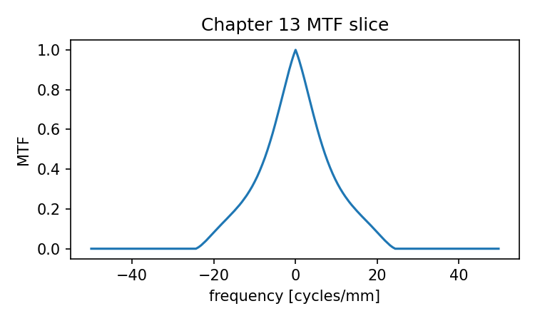
Source and validation note

The OTF/MTF formulas here assume incoherent, shift-invariant imaging and a properly normalized PSF. Real optical-design software may compute diffraction MTF, geometric MTF, polychromatic MTF, field-dependent curves, or direction-specific sagittal/tangential curves under additional conventions. The chapter keeps the core Fourier relationship visible before adding those production details.