Chapter 12: How PSF Is Computed from a Pupil Function

A point source should be the simplest possible object.

It has no size. It has no texture. It has no edge, no pattern, no detail. In geometric optics, a perfect lens would take all rays from that point and bring them back to one point in the image plane.

But real optical systems do not make mathematical points.

Even a perfect circular aperture spreads a point into a small diffraction pattern. Aberrations spread it further, deform it, shift energy out of the center, or produce asymmetric tails.

That spread-out image of a point is the point spread function, or PSF.

The previous chapter built the object that diffraction calculation needs:

$$P(x, y) = A(x, y)\exp\left(i\frac{2\pi W(x, y)}{\lambda}\right)$$

This is the complex pupil function. It stores aperture amplitude and wavefront phase.

Now we let that pupil function form an image.

The short computational chain is:

complex pupil function
→ Fourier transform
→ complex image-plane field
→ squared magnitude
→ PSF

In code, the skeleton is short:

field = np.fft.fftshift(np.fft.fft2(np.fft.ifftshift(pupil)))
psf = np.abs(field) ** 2
psf = psf / np.sum(psf)

Those three lines are the center of this chapter.

But they are not magic. We need to unpack what they mean, what assumptions they use, and what can go wrong.

1. What the PSF represents

The PSF is the intensity distribution produced in the image plane by a point object.

If the optical system were perfect and there were no diffraction, the PSF would be an infinitely small point. But physical light has wavelength, and apertures have finite size. A finite aperture cannot focus light into an infinitely small spot.

For a circular, aberration-free pupil, the ideal diffraction pattern is the familiar Airy pattern:

• a bright central core;
• surrounding rings;
• decreasing intensity away from the center.

This is the diffraction-limited PSF.

When aberrations are present, the pupil phase is no longer flat. The Fourier transform of that distorted complex pupil redistributes energy in the image plane. The PSF changes shape.

So the PSF is not merely a pretty picture. It answers a concrete imaging question:

If the object contains one ideal point, what intensity pattern does the system draw in the image?

Once we know that, we are very close to understanding blur, resolution, and MTF.

2. From pupil plane to image plane

The pupil function lives in the pupil plane. It tells us the complex field across the aperture.

The PSF lives in the image plane. It tells us the intensity around the focused point image.

Under the usual scalar Fraunhofer diffraction approximation, the complex field in the focal region is proportional to the Fourier transform of the pupil function:

$$U(\xi, \eta) \propto \mathcal{F}{P(x, y)}$$

The PSF is the squared magnitude of that complex field:

$$\mathrm{PSF}(\xi, \eta) = |U(\xi, \eta)|^2$$

Combining the two:

$$\mathrm{PSF}(\xi, \eta) \propto \left|\mathcal{F}{P(x, y)}\right|^2$$

where:

• $P(x,y)$ is the complex pupil function;
• $U(\xi,\eta)$ is the complex image-plane field;
• $\xi,\eta$ are image-plane or angular coordinates;
• $\mathcal{F}$ denotes a Fourier transform.

The proportionality sign matters. A real physical PSF needs correct coordinate scaling and energy normalization. For learning the computational chain, we can first compute a normalized PSF:

$$\sum_{\xi,\eta}\mathrm{PSF}(\xi,\eta)=1$$

That means the PSF is treated as an energy distribution. The total energy is one, and we study where that energy goes.

This normalization is simple and useful:

psf = psf / np.sum(psf)

It does not solve every physical scaling problem, but it makes comparisons between different pupil functions much clearer.

3. Why the Fourier transform appears

The Fourier transform appears because the image-plane field is built by coherent addition of contributions from all pupil points.

Each point in the pupil contributes a small wave. In the far field or focal plane approximation, the phase relationship between those contributions changes with image-plane position. The Fourier transform is the mathematical operation that sums all those complex contributions for each output position.

This is the part that ray diagrams hide.

A ray diagram says:

This part of the pupil sends light in this direction.

A diffraction calculation says:

All pupil points contribute complex amplitudes, and these amplitudes interfere.

The PSF is produced by interference.

That is why the pupil function must be complex. If we only kept OPD as a real-valued map, we would know wavefront error, but we would not yet have the object needed for coherent summation.

The chain now looks like this:

OPD map
→ phase map
→ complex pupil function
→ coherent Fourier summation
→ image-plane intensity

This is the moment where wavefront error becomes visible blur.

4. A perfect circular pupil

Start with the simplest case: a clear circular aperture with no aberration.

Inside the pupil:

$$A(x,y)=1$$

$$W(x,y)=0$$

So:

$$P(x,y)=1$$

Outside the pupil:

$$P(x,y)=0$$

This flat circular pupil produces the diffraction-limited Airy pattern.

Let us reuse the pupil grid idea from the previous chapter.

import numpy as np
import matplotlib.pyplot as plt


def make_pupil_grid(n=256):
    coord = np.linspace(-1.0, 1.0, n)
    x, y = np.meshgrid(coord, coord)

    rho = np.sqrt(x**2 + y**2)
    theta = np.arctan2(y, x)
    mask = rho <= 1.0

    return x, y, rho, theta, mask


def pupil_function_from_opd(opd, mask, wavelength, amplitude=None):
    if amplitude is None:
        amplitude = mask.astype(float)

    phase = 2.0 * np.pi * opd / wavelength
    pupil = amplitude * np.exp(1j * phase)

    pupil[~mask] = 0.0 + 0.0j

    return pupil, phase

Now create a perfect pupil:

wavelength = 550e-9  # meters

x, y, rho, theta, mask = make_pupil_grid(n=256)

zero_opd = np.zeros_like(rho)

perfect_pupil, perfect_phase = pupil_function_from_opd(
    opd=zero_opd,
    mask=mask,
    wavelength=wavelength
)

The pupil is complex, but in this perfect case its phase is zero inside the aperture. So the complex value is simply:

$$1 + 0i$$

inside the circle.

Now we are ready to compute the PSF.

5. Computing a PSF with FFT

A discrete Fourier transform is computed with numpy.fft.fft2.

Because we usually want the central peak in the middle of the displayed image, we use fftshift.

A careful version uses ifftshift before the transform and fftshift after it:

def compute_psf(pupil, normalize=True):
    """
    Compute a normalized PSF from a complex pupil function.

    Parameters
    ----------
    pupil : 2D complex array
        Complex pupil function.
    normalize : bool
        If True, normalize total PSF energy to 1.

    Returns
    -------
    psf : 2D array
        Intensity PSF.
    field : 2D complex array
        Complex field in the image plane.
    """
    field = np.fft.fftshift(
        np.fft.fft2(
            np.fft.ifftshift(pupil)
        )
    )

    psf = np.abs(field) ** 2

    if normalize:
        total = np.sum(psf)
        if total > 0:
            psf = psf / total

    return psf, field

Run it:

perfect_psf, perfect_field = compute_psf(perfect_pupil)

This perfect_psf array is the diffraction-limited PSF for our sampled circular pupil.

It is not yet labeled in micrometers or arcseconds. It is a sampled Fourier-plane result. We will return to coordinate scaling later in the chapter.

First, look at the pattern.

6. Displaying the PSF

A PSF usually has a very bright central peak and much weaker surrounding structure. If you display it linearly, the center may dominate so strongly that the rings are hard to see.

So we often display both:

1. linear intensity;
2. logarithmic intensity.

def show_psf(psf, title="PSF"):
    plt.figure(figsize=(5, 4))
    plt.imshow(psf, origin="lower")
    plt.colorbar(label="Normalized intensity")
    plt.title(title + " - linear scale")
    plt.xlabel("Image sample x")
    plt.ylabel("Image sample y")
    plt.tight_layout()
    plt.show()

    plt.figure(figsize=(5, 4))
    plt.imshow(np.log10(psf + 1e-12), origin="lower")
    plt.colorbar(label="log10 intensity")
    plt.title(title + " - log scale")
    plt.xlabel("Image sample x")
    plt.ylabel("Image sample y")
    plt.tight_layout()
    plt.show()


show_psf(perfect_psf, title="Diffraction-limited circular pupil")

The logarithmic plot is not a different PSF. It is the same PSF shown with a display transform.

This distinction matters. A log-scale PSF can make weak rings look visually important. A linear-scale PSF can hide structure that still affects MTF. Good analysis often needs both views.

A sensible habit is:

Use linear scale to judge energy concentration.
Use log scale to inspect weak structure.

The central peak is usually the most important part for sharpness, but the faint surrounding energy tells you where contrast has gone.

7. Zero padding: making the displayed PSF smoother

The FFT output sampling depends on the input array size. If the pupil array is small, the PSF may look blocky or under-sampled.

A common technique is to zero-pad the pupil before the FFT.

Zero padding does not add new optical information. It interpolates the Fourier-domain display more finely.

Here is a padded PSF function:

def pad_array_centered(array, pad_factor=2):
    """
    Zero-pad a 2D array around its center.

    Parameters
    ----------
    array : 2D array
        Input array.
    pad_factor : int
        Output size will be pad_factor times the input size.

    Returns
    -------
    padded : 2D array
        Centered zero-padded array.
    """
    if pad_factor == 1:
        return array

    n, m = array.shape
    new_n = n * pad_factor
    new_m = m * pad_factor

    padded = np.zeros((new_n, new_m), dtype=array.dtype)

    start_n = (new_n - n) // 2
    start_m = (new_m - m) // 2

    padded[start_n:start_n + n, start_m:start_m + m] = array

    return padded


def compute_psf(pupil, pad_factor=2, normalize=True):
    """
    Compute a PSF from a complex pupil function, with optional zero padding.
    """
    padded_pupil = pad_array_centered(pupil, pad_factor=pad_factor)

    field = np.fft.fftshift(
        np.fft.fft2(
            np.fft.ifftshift(padded_pupil)
        )
    )

    psf = np.abs(field) ** 2

    if normalize:
        total = np.sum(psf)
        if total > 0:
            psf = psf / total

    return psf, field

Now compute a smoother display:

perfect_psf, perfect_field = compute_psf(
    perfect_pupil,
    pad_factor=4
)

show_psf(perfect_psf, title="Diffraction-limited PSF with zero padding")

Again, zero padding is not magic resolution. It gives us more output samples between the same physical features.

A useful way to say it:

Zero padding makes the plotted PSF smoother.
It does not make the optical system sharper.

That sentence prevents many bad interpretations.

8. Reading the perfect PSF

The perfect circular-pupil PSF has three major features.

First, the central peak is compact and symmetric. This is the Airy core.

Second, rings surround the central peak. These rings are not aberrations. They are diffraction from a finite circular aperture.

Third, the pattern is radially symmetric because the pupil is radially symmetric and the phase is flat.

This is an important baseline.

If the optical system has a circular clear aperture and no aberration, the PSF is not a point. It is already spread out by diffraction.

So when someone says “diffraction-limited,” they do not mean “infinitely sharp.” They mean the system is limited mainly by diffraction rather than aberration.

In practice:

perfect wavefront + finite aperture
→ diffraction-limited PSF

distorted wavefront + finite aperture
→ aberrated PSF

A PSF can only be judged correctly relative to this baseline. The right comparison is not against a mathematical point. The right comparison is against the diffraction-limited PSF for the same aperture and wavelength.

9. Adding aberration

Now let us reuse a synthetic OPD map. We will make a defocus-like and astigmatism-like wavefront, just as in the previous chapter.

def synthetic_opd(rho, theta, mask, wavelength):
    """
    Create a synthetic OPD map in meters.

    This is a teaching wavefront, not a full optical design result.
    """
    opd = np.zeros_like(rho)

    defocus = 0.50 * wavelength
    astigmatism = 0.25 * wavelength

    opd += defocus * (2.0 * rho**2 - 1.0)
    opd += astigmatism * rho**2 * np.cos(2.0 * theta)

    opd[~mask] = 0.0

    return opd

Build the aberrated pupil:

aberrated_opd = synthetic_opd(
    rho=rho,
    theta=theta,
    mask=mask,
    wavelength=wavelength
)

aberrated_pupil, aberrated_phase = pupil_function_from_opd(
    opd=aberrated_opd,
    mask=mask,
    wavelength=wavelength
)

aberrated_psf, aberrated_field = compute_psf(
    aberrated_pupil,
    pad_factor=4
)

Now display it:

show_psf(aberrated_psf, title="Aberrated PSF")

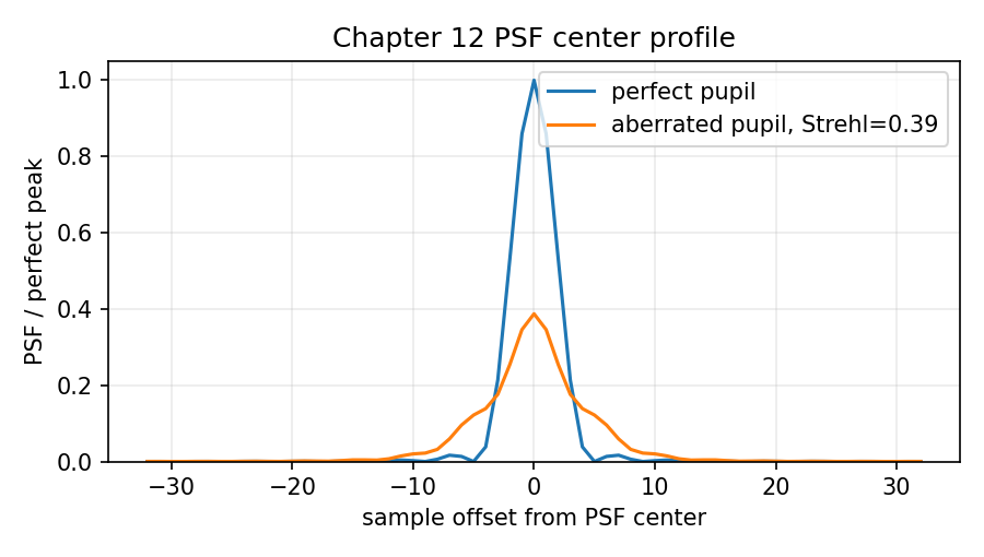
Compared with the perfect PSF, the aberrated PSF should show energy redistributed away from the center. Depending on the aberration, the central peak may broaden, become asymmetric, or develop side structure.

This is the central visual lesson of the chapter:

Aberration is phase error in the pupil.
The PSF shows where that phase error sends the image energy.

A wavefront map may look abstract. The PSF shows its consequence.

10. Comparing perfect and aberrated PSFs

A side-by-side display is useful.

def show_two_psfs(psf_a, psf_b, title_a, title_b, log_scale=False):
    if log_scale:
        image_a = np.log10(psf_a + 1e-12)
        image_b = np.log10(psf_b + 1e-12)
        label = "log10 intensity"
    else:
        image_a = psf_a
        image_b = psf_b
        label = "Normalized intensity"

    vmin = min(np.nanmin(image_a), np.nanmin(image_b))
    vmax = max(np.nanmax(image_a), np.nanmax(image_b))

    plt.figure(figsize=(10, 4))

    plt.subplot(1, 2, 1)
    plt.imshow(image_a, origin="lower", vmin=vmin, vmax=vmax)
    plt.colorbar(label=label)
    plt.title(title_a)
    plt.xlabel("Image sample x")
    plt.ylabel("Image sample y")

    plt.subplot(1, 2, 2)
    plt.imshow(image_b, origin="lower", vmin=vmin, vmax=vmax)
    plt.colorbar(label=label)
    plt.title(title_b)
    plt.xlabel("Image sample x")
    plt.ylabel("Image sample y")

    plt.tight_layout()
    plt.show()


show_two_psfs(
    perfect_psf,
    aberrated_psf,
    "Perfect PSF",
    "Aberrated PSF",
    log_scale=False
)

show_two_psfs(
    perfect_psf,
    aberrated_psf,
    "Perfect PSF",
    "Aberrated PSF",
    log_scale=True
)

The linear comparison tells us how much energy remains concentrated near the center.

The log comparison shows faint structure.

Both matter. If the central energy drops, fine detail contrast usually suffers. If faint energy spreads far away, the image can gain halos or low-level blur.

This is why PSF is more informative than a single number. It shows the spatial shape of the blur.

MTF, which we will compute in the next chapter, compresses this spatial information into frequency response. That is powerful, but it also hides some visible structure. The PSF lets us see the blur directly.

11. Encircled energy: a simple PSF summary

Before going to MTF, it is useful to introduce one simple PSF-based summary: encircled energy.

Encircled energy asks:

How much of the total PSF energy lies inside a given radius?

This is not the same as MTF, but it is often useful. A sharper PSF concentrates energy into a smaller radius.

Here is a simple implementation in pixel units:

def encircled_energy(psf):
    """
    Compute encircled energy as a function of radius in pixel units.

    Parameters
    ----------
    psf : 2D array
        Normalized PSF.

    Returns
    -------
    radii : 1D array
        Radius values in pixels.
    energy : 1D array
        Encircled energy for each radius.
    """
    n, m = psf.shape
    cy = (n - 1) / 2.0
    cx = (m - 1) / 2.0

    yy, xx = np.indices(psf.shape)
    r = np.sqrt((xx - cx)**2 + (yy - cy)**2)

    r_flat = r.ravel()
    psf_flat = psf.ravel()

    order = np.argsort(r_flat)
    r_sorted = r_flat[order]
    psf_sorted = psf_flat[order]

    cumulative = np.cumsum(psf_sorted)

    return r_sorted, cumulative

Plot perfect versus aberrated:

r_perfect, e_perfect = encircled_energy(perfect_psf)
r_aberr, e_aberr = encircled_energy(aberrated_psf)

plt.figure(figsize=(6, 4))
plt.plot(r_perfect, e_perfect, label="Perfect")
plt.plot(r_aberr, e_aberr, label="Aberrated")
plt.xlabel("Radius [pixels]")
plt.ylabel("Encircled energy")
plt.title("Encircled energy comparison")
plt.legend()
plt.grid(True)
plt.tight_layout()
plt.show()

If the aberrated PSF spreads energy outward, its encircled energy curve rises more slowly.

This gives us a simple way to say:

The aberrated system needs a larger radius to contain the same fraction of point-source energy.

Again, this is not a replacement for MTF. It is another way of looking at image formation.

PSF is spatial. Encircled energy summarizes spatial concentration. MTF will describe spatial frequency response.

They are connected, but they are not identical.

12. Strehl ratio: central peak as a warning light

Another common PSF-based quantity is the Strehl ratio.

In simple computational terms, Strehl ratio compares the peak intensity of an aberrated PSF with the peak intensity of the diffraction-limited PSF, under matching normalization and sampling:

$$S = \frac{\max(\mathrm{PSF}$$\text{aberrated})} {\max(\mathrm{PSF}\text{diffraction-limited})}

Code:

def strehl_ratio(aberrated_psf, perfect_psf):
    return np.max(aberrated_psf) / np.max(perfect_psf)


strehl = strehl_ratio(aberrated_psf, perfect_psf)
print(strehl)

A lower Strehl ratio means the central peak has lost energy relative to the ideal diffraction-limited case.

This is a useful warning light, but it is not a full image-quality description.

Two PSFs can have similar peak values but different shapes. One may have symmetric broadening; another may have a comet-like tail. Their visual effects can differ.

So the rule is:

Strehl ratio summarizes the central peak.
The PSF image shows the whole blur structure.

The PSF still deserves to be looked at.

13. Why spot diagrams and PSFs are different

At this point, it is worth comparing PSF with the spot diagram from earlier chapters.

A spot diagram comes from traced rays. It shows where rays intersect the image plane.

A PSF comes from diffraction calculation. It uses the complex pupil function, including phase, and computes interference.

They may tell similar stories for badly aberrated systems, but they are not the same calculation.

A spot diagram answers:

Where do sampled rays land?

A PSF answers:

What intensity distribution does a point source produce after wave interference?

For large aberrations, the geometric spot can give a useful first impression of blur. But near the diffraction limit, a spot diagram can be misleading. It may show a tight ray bundle and still fail to show diffraction rings. It also does not directly tell us how energy is distributed by interference.

This is one reason optical software provides multiple plots:

• spot diagram;
• ray fan;
• OPD;
• PSF;
• MTF.

They are not redundant. They are different projections of the same optical system.

The full computational route matters:

ray tracing
→ OPD
→ pupil function
→ PSF

The spot diagram branches off from ray intersections. The PSF branches off from wavefront phase.

That difference is the heart of Part Four of this book.

14. The Airy pattern and the diffraction limit

For a perfect circular aperture, the analytic PSF is the Airy pattern. Its intensity profile is commonly written in terms of a Bessel function. We do not need the full analytic derivation here, but we should know the practical meaning.

The first dark ring occurs at an angular radius approximately:

$$\theta \approx 1.22\frac{\lambda}{D}$$

where:

• $\theta$ is angular radius in radians;
• $\lambda$ is wavelength;
• $D$ is aperture diameter.

At the focal plane, the corresponding radius is approximately:

$$r \approx 1.22\lambda N$$

where $N$ is the f-number.

This tells us something physically important:

Longer wavelength gives a larger diffraction spot.
Smaller aperture diameter gives a larger diffraction spot.
Larger f-number gives a larger diffraction spot.

This is why stopping down a lens can improve aberrations but worsen diffraction blur. The PSF is shaped by both aberration and aperture size.

Our FFT computation has reproduced the structure of the Airy pattern from the pupil function. To assign physical units to the output samples, we need aperture size, focal length, wavelength, and sampling relationships. That full scaling is important in engineering use, but the core generation mechanism is already visible:

clear circular pupil
→ Fourier transform
→ Airy-like PSF

That is the computational fact we needed first.

15. Coordinate scaling: what the FFT output means

The FFT returns samples in a frequency-like coordinate. If the pupil coordinate is normalized, the output coordinate is also in a normalized reciprocal coordinate. That is fine for comparing shapes, but physical interpretation needs scaling.

For a physical aperture field sampled over pupil coordinates $X,Y$, the focal-plane coordinates are related to diffraction angles. Roughly:

$$\theta_x \sim \lambda f_x$$

$$\theta_y \sim \lambda f_y$$

where $f_x,f_y$ are spatial frequency coordinates associated with the pupil-plane sampling.

At the focal plane of a lens with focal length $F$:

$$X_\text{image} \sim F\theta_x$$

$$Y_\text{image} \sim F\theta_y$$

The exact implementation depends on how you sampled the physical pupil and how you define the Fourier transform normalization.

For this chapter, the safest practical division is:

First compute the correct normalized PSF shape.
Then attach physical coordinates using known aperture sampling, wavelength, and focal length.

Trying to do both at once often confuses beginners.

Here is a simple coordinate helper for a physical pupil diameter:

def psf_angular_coordinates(n_output, pupil_sample_spacing, wavelength):
    """
    Estimate angular coordinates for FFT-based Fraunhofer PSF.

    Parameters
    ----------
    n_output : int
        Number of samples in the padded pupil / PSF array.
    pupil_sample_spacing : float
        Physical pupil-plane sample spacing, in meters.
    wavelength : float
        Wavelength, in meters.

    Returns
    -------
    theta : 1D array
        Angular coordinate samples, in radians.
    """
    freq = np.fft.fftshift(
        np.fft.fftfreq(n_output, d=pupil_sample_spacing)
    )

    theta = wavelength * freq

    return theta

If your original pupil diameter is $D$, and the unpadded pupil grid has $n$ samples across the full square coordinate range, a rough sample spacing is:

pupil_sample_spacing = D / n

Then:

D = 5e-3  # 5 mm aperture diameter
n_input = perfect_pupil.shape[0]
pad_factor = 4
n_output = n_input * pad_factor

dx_pupil = D / n_input
theta = psf_angular_coordinates(
    n_output=n_output,
    pupil_sample_spacing=dx_pupil,
    wavelength=wavelength
)

This gives angular samples in radians. If the focal length is known, convert to focal-plane length:

focal_length = 50e-3  # 50 mm
image_coord = focal_length * theta

This coordinate scaling is useful, but it also deserves caution. The more realistic your model becomes, the more carefully you must define:

• pupil diameter;
• entrance pupil versus exit pupil;
• focal length;
• image-space refractive index;
• sampling convention;
• FFT normalization;
• field point;
• wavelength.

For now, remember the main warning:

The PSF array is easy to compute.
The physical coordinate labels require careful bookkeeping.

Chapter 14 will return to sampling and normalization more aggressively.

16. A complete minimal PSF script

Here is a compact script that builds both perfect and aberrated PSFs.

import numpy as np
import matplotlib.pyplot as plt


def make_pupil_grid(n=256):
    coord = np.linspace(-1.0, 1.0, n)
    x, y = np.meshgrid(coord, coord)

    rho = np.sqrt(x**2 + y**2)
    theta = np.arctan2(y, x)
    mask = rho <= 1.0

    return x, y, rho, theta, mask


def synthetic_opd(rho, theta, mask, wavelength):
    opd = np.zeros_like(rho)

    defocus = 0.50 * wavelength
    astigmatism = 0.25 * wavelength

    opd += defocus * (2.0 * rho**2 - 1.0)
    opd += astigmatism * rho**2 * np.cos(2.0 * theta)

    opd[~mask] = 0.0

    return opd


def pupil_function_from_opd(opd, mask, wavelength, amplitude=None):
    if amplitude is None:
        amplitude = mask.astype(float)

    phase = 2.0 * np.pi * opd / wavelength
    pupil = amplitude * np.exp(1j * phase)

    pupil[~mask] = 0.0 + 0.0j

    return pupil, phase


def pad_array_centered(array, pad_factor=2):
    if pad_factor == 1:
        return array

    n, m = array.shape
    new_n = n * pad_factor
    new_m = m * pad_factor

    padded = np.zeros((new_n, new_m), dtype=array.dtype)

    start_n = (new_n - n) // 2
    start_m = (new_m - m) // 2

    padded[start_n:start_n + n, start_m:start_m + m] = array

    return padded


def compute_psf(pupil, pad_factor=4, normalize=True):
    padded_pupil = pad_array_centered(pupil, pad_factor=pad_factor)

    field = np.fft.fftshift(
        np.fft.fft2(
            np.fft.ifftshift(padded_pupil)
        )
    )

    psf = np.abs(field) ** 2

    if normalize:
        total = np.sum(psf)
        if total > 0:
            psf = psf / total

    return psf, field


def show_two_psfs(psf_a, psf_b, title_a, title_b, log_scale=False):
    if log_scale:
        image_a = np.log10(psf_a + 1e-12)
        image_b = np.log10(psf_b + 1e-12)
        label = "log10 intensity"
    else:
        image_a = psf_a
        image_b = psf_b
        label = "Normalized intensity"

    vmin = min(np.nanmin(image_a), np.nanmin(image_b))
    vmax = max(np.nanmax(image_a), np.nanmax(image_b))

    plt.figure(figsize=(10, 4))

    plt.subplot(1, 2, 1)
    plt.imshow(image_a, origin="lower", vmin=vmin, vmax=vmax)
    plt.colorbar(label=label)
    plt.title(title_a)
    plt.xlabel("Image sample x")
    plt.ylabel("Image sample y")

    plt.subplot(1, 2, 2)
    plt.imshow(image_b, origin="lower", vmin=vmin, vmax=vmax)
    plt.colorbar(label=label)
    plt.title(title_b)
    plt.xlabel("Image sample x")
    plt.ylabel("Image sample y")

    plt.tight_layout()
    plt.show()


wavelength = 550e-9

x, y, rho, theta, mask = make_pupil_grid(n=256)

zero_opd = np.zeros_like(rho)
perfect_pupil, _ = pupil_function_from_opd(
    opd=zero_opd,
    mask=mask,
    wavelength=wavelength
)

aberrated_opd = synthetic_opd(
    rho=rho,
    theta=theta,
    mask=mask,
    wavelength=wavelength
)

aberrated_pupil, _ = pupil_function_from_opd(
    opd=aberrated_opd,
    mask=mask,
    wavelength=wavelength
)

perfect_psf, _ = compute_psf(perfect_pupil, pad_factor=4)
aberrated_psf, _ = compute_psf(aberrated_pupil, pad_factor=4)

show_two_psfs(
    perfect_psf,
    aberrated_psf,
    "Perfect PSF",
    "Aberrated PSF",
    log_scale=False
)

show_two_psfs(
    perfect_psf,
    aberrated_psf,
    "Perfect PSF",
    "Aberrated PSF",
    log_scale=True
)

strehl = np.max(aberrated_psf) / np.max(perfect_psf)
print("Approximate Strehl ratio:", strehl)

This script is still a teaching model. It does not replace a full optical design package. But it exposes the calculation skeleton clearly:

make pupil
→ add phase from OPD
→ FFT
→ square magnitude
→ normalize
→ compare

That is exactly the hidden step we wanted to open.

17. Connecting this to Optiland

In a real Optiland workflow, you would usually not hand-create the OPD map from a synthetic polynomial. You would define or load an optical system, select a field point and wavelength, and then ask the analysis tools for wavefront or PSF results.

Conceptually, the flow is:

Optiland optical system
→ ray tracing and wavefront analysis
→ pupil function or equivalent internal representation
→ PSF analysis

A validation-style comparison workflow looks like this:

# Version-checked workflow outline.
# Check your installed Optiland version for exact API names.

# 1. Build or load an optical system.
# optic = ...

# 2. Select field and wavelength.
# field = ...
# wavelength = ...

# 3. Compute wavefront / OPD using Optiland analysis tools.
# wavefront = ...
# opd = wavefront.opd_map(...)

# 4. Build a pupil function from that OPD.
# pupil, phase = pupil_function_from_opd(opd, mask, wavelength)

# 5. Compute a teaching PSF using NumPy.
# psf_numpy, field_numpy = compute_psf(pupil, pad_factor=4)

# 6. Compute PSF using Optiland's own PSF analysis.
# psf_optiland = ...

# 7. Compare shape, normalization, sampling, and coordinate scaling.

Twenty lines of NumPy do not replace a mature optical design tool. They make the hidden calculation inspectable.

When Optiland gives you a PSF, you should now be able to ask:

• What pupil was sampled?
• What wavelength was used?
• What field point was used?
• What OPD or phase was included?
• What aperture mask was applied?
• What FFT sampling and normalization were used?
• Is the plot linear or logarithmic?
• Are the coordinates image-plane, angular, or normalized?

These questions are more valuable than memorizing a button sequence.

A tool can produce the PSF. Understanding means knowing what had to happen for that PSF to exist.

18. Common mistakes in PSF calculation

Mistake 1: Taking the Fourier transform of OPD directly

OPD is not the pupil function.

Wrong:

psf = np.abs(np.fft.fft2(opd)) ** 2

Correct:

phase = 2.0 * np.pi * opd / wavelength
pupil = amplitude * np.exp(1j * phase)
psf = np.abs(np.fft.fft2(pupil)) ** 2

The FFT operates on the complex field, not on OPD as a height map.

Mistake 2: Forgetting to square the magnitude

The Fourier transform gives a complex field. The PSF is intensity.

Wrong:

psf = np.fft.fft2(pupil)

Correct:

field = np.fft.fft2(pupil)
psf = np.abs(field) ** 2

Intensity is squared magnitude.

Mistake 3: Comparing unnormalized PSFs

If two PSFs have different total sums, peak comparisons can be misleading.

Better:

psf = psf / np.sum(psf)

Then you can compare energy distribution more fairly.

Mistake 4: Believing zero padding increases resolution

Zero padding makes the PSF display smoother. It does not improve the physical optical resolution.

Mistake 5: Ignoring display scale

A linear plot and a log plot can make the same PSF feel very different.

Always check which scale is being used before interpreting rings, halos, or faint tails.

Mistake 6: Forgetting that PSF depends on wavelength and field

A PSF is not a universal property of a lens.

It depends on:

• wavelength;
• field point;
• focus position;
• aperture;
• pupil sampling;
• polarization assumptions if included;
• aberration state.

A single PSF plot is one slice through a larger optical behavior.

19. What this chapter adds to the full chain

We can now extend the computation chain:

lens prescription
→ surfaces and materials
→ ray tracing
→ optical path length
→ OPD map
→ pupil amplitude and phase
→ complex pupil function
→ Fourier transform
→ PSF

The new step is:

$$\mathrm{PSF} = \left|\mathcal{F}{P(x,y)}\right|^2$$

with normalization applied for practical comparison.

That is a major milestone.

We have moved from geometric rays to a wave-optical image of a point. We have also seen why a point never remains a point in a real optical system.

A clear circular pupil produces a diffraction-limited Airy-like pattern. An aberrated pupil changes phase across the aperture and redistributes energy in the PSF. An obstructed or apodized pupil changes amplitude and also changes the PSF.

The PSF is where aperture, diffraction, and aberration meet in image space.

The next chapter will take one more step. Instead of asking how one point is blurred, we will ask how different spatial frequencies are transmitted.

That takes us from PSF to OTF, and then to MTF.

The MTF curve that looked like a software output in Chapter 1 is now almost within reach.

Chapter summary

The PSF is the image-plane intensity distribution produced by an ideal point source.

Under the usual scalar Fraunhofer diffraction approximation, the complex image-plane field is proportional to the Fourier transform of the complex pupil function:

$$U(\xi,\eta) \propto \mathcal{F}{P(x,y)}$$

The PSF is the squared magnitude of that field:

$$\mathrm{PSF}(\xi,\eta) = |U(\xi,\eta)|^2$$

In minimal NumPy code:

field = np.fft.fftshift(np.fft.fft2(np.fft.ifftshift(pupil)))
psf = np.abs(field) ** 2
psf = psf / np.sum(psf)

A perfect clear circular pupil produces a diffraction-limited Airy-like PSF. An aberrated pupil redistributes energy away from the ideal central peak. A changed aperture amplitude also changes the PSF, even if the wavefront phase is flat.

The PSF should be inspected carefully, often in both linear and logarithmic display. Zero padding can make the displayed PSF smoother, but it does not improve the actual optical resolution.

Most importantly, the FFT must be applied to the complex pupil function, not directly to the OPD map.

The computation chain now reaches:

OPD
→ pupil function
→ PSF

Next, we will ask how this PSF acts on image detail at different spatial frequencies. That question leads to the OTF and MTF.

Generated validation figure

Source and validation note

The PSF computation in this chapter uses the scalar Fourier-optics model appropriate for teaching the pupil-to-image calculation. It deliberately omits vector diffraction, polarization effects, partial coherence, detector sampling, and detailed physical units. Those omissions are boundaries of the chapter, not claims that those effects are unimportant.