Chapter 11: Pupil Function: Writing the Wavefront as Complex Numbers

At the end of the previous chapter, OPD gave us a new kind of information.

A spot diagram tells us where rays land. A ray fan tells us how real rays deviate from a reference. OPD tells us something more subtle: for each point in the pupil, how far ahead or behind that part of the wavefront is compared with the ideal reference wavefront.

That is already a big step. But OPD by itself is still not ready to make an image.

To compute a diffraction PSF, the computer needs to know how light from the whole pupil interferes at the image plane. That means it needs two things at each pupil point:

1. How much light gets through.
2. What phase that light has.

These two pieces are exactly what the pupil function stores.

The pupil function is the moment where wavefront error becomes a complex-valued array. It is the bridge between geometric optical path error and Fourier optics.

This chapter is short in concept but important in the chain:

OPD map
→ pupil amplitude
→ pupil phase
→ complex pupil function
→ PSF

The next chapter will take the Fourier transform of this complex pupil function and turn it into a PSF. Here, we prepare the input carefully.

Do not rush this step. Many wrong PSF and MTF calculations begin with a pupil function that was built with the wrong units, the wrong mask, or the wrong sign convention.

1. The black box we are opening

A diffraction calculation often appears in books as one elegant line:

PSF is related to the Fourier transform of the pupil function.

That statement is true under the usual Fraunhofer approximation, but it hides a practical question:

What exactly is the pupil function in code?

It is not just the aperture shape.

It is not just the OPD map.

It is not just a phase image.

It is a complex-valued function over the pupil:

$$P(x, y) = A(x, y)\exp\left(i\frac{2\pi W(x, y)}{\lambda}\right)$$

where:

• $P(x, y)$ is the complex pupil function.
• $A(x, y)$ is the pupil amplitude.
• $W(x, y)$ is the OPD or wavefront error.
• $\lambda$ is the wavelength.
• $i$ is the imaginary unit.
• $x, y$ are pupil coordinates.

This formula is the whole chapter in one line.

But one line is not enough. We need to know what each part means, how to sample it, and how to write it without lying to ourselves.

2. The aperture mask: where light exists

Start with the simplest part: the aperture.

For an ideal circular pupil, light passes through points inside a circle and is blocked outside it. In normalized pupil coordinates, we can write:

$$\rho = \sqrt{x^2 + y^2}$$

Inside the pupil:

$$\rho \leq 1$$

Outside the pupil:

$$\rho > 1$$

So the simplest aperture mask is:

$$M(x, y) = \begin{cases} 1, & \rho \leq 1 \ 0, & \rho > 1 \end{cases}$$

This mask is not yet the full pupil function. It only says where light is allowed to pass.

In code, this becomes a boolean array:

mask = rho <= 1.0

That one line matters. Without it, your FFT will include light from outside the pupil. The result may still look like a pattern, but it is no longer the PSF of the optical system you intended to model.

This is a useful habit in computational optics:

A wrong array can still produce a beautiful image.

The computer does not know whether your pupil is physical. It only executes the numbers you give it.

3. Pupil amplitude: not always just 1

For a clear, ideal, uniformly illuminated circular aperture, the amplitude is usually written as:

$$A(x, y) = M(x, y)$$

That means:

• amplitude is 1 inside the pupil;
• amplitude is 0 outside the pupil.

This is the simplest case, and it is the right place to begin.

But in real optical systems, amplitude can be more complicated. It may include:

• vignetting;
• central obstruction;
• spider vanes in telescopes;
• transmission variation;
• apodization;
• polarization-dependent effects;
• coating or material transmission differences.

For example, a telescope with a central obstruction has a mask like this:

$$M(x, y) = \begin{cases} 1, & r_\text{inner} < \rho \leq 1 \ 0, & \text{otherwise} \end{cases}$$

A system with apodization might have a smooth amplitude such as:

$$A(\rho) = \exp(-\alpha \rho^2)$$

inside the aperture.

For this chapter, we will mostly use the simple circular pupil. But it is important to keep the distinction clear:

mask: where light is allowed
amplitude: how much field amplitude passes through
intensity: amplitude squared

Amplitude is not intensity. If intensity transmission is $T$, then field amplitude is usually proportional to:

$$A = \sqrt{T}$$

That square root is a common source of mistakes. If you put intensity directly into a field amplitude array, your PSF energy will be wrong.

For now, we will keep:

amplitude = mask.astype(float)

That is enough to build the first pupil function.

4. OPD becomes phase

The OPD map tells us how much optical path difference each pupil point has.

If the OPD at one point is $W(x,y)$, then the corresponding phase is:

$$\phi(x, y) = \frac{2\pi W(x, y)}{\lambda}$$

This is the key conversion.

The unit rule is simple but strict:

W and λ must use the same length unit.

If $W$ is in meters, $\lambda$ must be in meters.

If $W$ is in micrometers, $\lambda$ must be in micrometers.

If $W$ is in nanometers and $\lambda$ is in meters, the code will still run, but the phase will be wrong by a factor of $10^9$. There is no warning. There is only a bad result.

Let us make the physical meaning concrete.

Suppose the wavelength is:

$$\lambda = 550\text{ nm}$$

If OPD is one full wavelength:

$$W = \lambda$$

then:

$$\phi = \frac{2\pi\lambda}{\lambda} = 2\pi$$

That point has completed one full phase cycle.

If OPD is half a wavelength:

$$W = \frac{\lambda}{2}$$

then:

$$\phi = \pi$$

That point is half a cycle out of phase.

This is why a small OPD can matter so much. A few hundred nanometers is tiny mechanically, but optically it can be a large fraction of a visible wavelength.

The pupil function stores this phase as a complex number:

$$\exp(i\phi) = \cos\phi + i\sin\phi$$

So the full pupil function becomes:

$$P(x, y) = A(x, y)\exp(i\phi(x, y))$$

or, substituting phase:

$$P(x, y) = A(x, y)\exp\left(i\frac{2\pi W(x, y)}{\lambda}\right)$$

This is the cleanest form to remember.

5. Why complex numbers are not decorative here

It is tempting to think of complex numbers as mathematical decoration. Here they are not decoration. They are how we store phase.

A real-valued OPD map says:

this pupil point is ahead or behind by this much optical path

A complex pupil function says:

this pupil point contributes this amplitude with this phase

When we later compute a PSF, light from different pupil points will interfere. Interference depends on phase.

Two parts of the pupil can have the same amplitude but opposite phase. They may partially cancel. Two parts can have aligned phase. They may reinforce.

That is why a spot diagram cannot fully replace a diffraction calculation. A spot diagram treats rays as landing points. A pupil function prepares the wave nature of light for coherent summation.

Here is the important shift:

Geometric ray tracing asks:
Where does this ray go?

Wave optics asks:
How do all pupil contributions add together as complex fields?

The pupil function is where we prepare the answer to the second question.

6. A minimal pupil grid

Now we write the first version in Python.

We will use normalized pupil coordinates. That means the pupil radius is 1, and the coordinate range is roughly:

x from -1 to 1
y from -1 to 1

This is not yet a physical length in millimeters. It is a normalized coordinate system. That is fine for this chapter because we are focusing on the conversion:

OPD → phase → complex pupil

Here is the grid:

import numpy as np
import matplotlib.pyplot as plt


def make_pupil_grid(n=256):
    """
    Create a square sampling grid with normalized pupil coordinates.

    Returns
    -------
    x, y : 2D arrays
        Normalized pupil coordinates.
    rho : 2D array
        Radial pupil coordinate.
    theta : 2D array
        Angular pupil coordinate.
    mask : 2D boolean array
        True inside the unit circular pupil.
    """
    coord = np.linspace(-1.0, 1.0, n)
    x, y = np.meshgrid(coord, coord)

    rho = np.sqrt(x**2 + y**2)
    theta = np.arctan2(y, x)
    mask = rho <= 1.0

    return x, y, rho, theta, mask

The output arrays all have shape:

(n, n)

A square grid is convenient for FFTs, even though the physical pupil is circular. The circular aperture is represented by the mask.

This is one of the first small compromises of numerical optics:

The computational array is square.
The optical aperture may not be.
The mask tells the array what is physically real.

That distinction will become very important in the next chapter.

7. A simple OPD map

In a real optical design program, OPD is computed from the optical system. Rays are traced through the surfaces, optical path length is accumulated, and the wavefront is compared with a reference sphere or reference wave.

For learning, we can begin with a synthetic OPD map. This lets us test the pupil function machinery without needing a full lens model in every example.

We will create a simple wavefront with two components:

1. Defocus-like variation.
2. Astigmatism-like variation.

This is not a full Zernike implementation. It is only a compact way to create a recognizable OPD pattern.

def synthetic_opd(rho, theta, mask, wavelength):
    """
    Create a synthetic OPD map in meters.

    This is a teaching wavefront, not a full optical design result.
    The coefficients are fractions of wavelength.
    """
    opd = np.zeros_like(rho)

    # Coefficients in meters
    defocus = 0.50 * wavelength
    astigmatism = 0.25 * wavelength

    # Simple wavefront terms
    opd += defocus * (2.0 * rho**2 - 1.0)
    opd += astigmatism * rho**2 * np.cos(2.0 * theta)

    # Outside the pupil, OPD is not physically meaningful.
    # We keep it at zero numerically, but the mask will block it.
    opd[~mask] = 0.0

    return opd

The important part is not the exact polynomial. The important part is that opd is an array with the same shape as the pupil grid.

Each sampled pupil point now has a wavefront error.

grid point → OPD value → phase value → complex pupil value

That is the conversion we want to make explicit.

8. Building the complex pupil function

Now we can write the function that does the main job of the chapter.

def pupil_function_from_opd(opd, mask, wavelength, amplitude=None):
    """
    Convert an OPD map into a complex pupil function.

    Parameters
    ----------
    opd : 2D array
        Optical path difference, in meters.
    mask : 2D boolean array
        True inside the aperture.
    wavelength : float
        Wavelength in meters.
    amplitude : 2D array or None
        Field amplitude transmission. If None, use a clear aperture.

    Returns
    -------
    pupil : 2D complex array
        Complex pupil function.
    phase : 2D array
        Phase in radians.
    """
    if amplitude is None:
        amplitude = mask.astype(float)

    phase = 2.0 * np.pi * opd / wavelength

    pupil = amplitude * np.exp(1j * phase)

    # Make sure the field is zero outside the aperture.
    pupil[~mask] = 0.0 + 0.0j

    return pupil, phase

This function is small, but it is doing a very important conversion.

Let us run it:

wavelength = 550e-9  # 550 nm, in meters

x, y, rho, theta, mask = make_pupil_grid(n=256)
opd = synthetic_opd(rho, theta, mask, wavelength)

pupil, phase = pupil_function_from_opd(
    opd=opd,
    mask=mask,
    wavelength=wavelength
)

At this point:

• opd is a real-valued array in meters.
• phase is a real-valued array in radians.
• pupil is a complex-valued array.

You can check:

print(opd.dtype)
print(phase.dtype)
print(pupil.dtype)

The third one should be complex.

Use this as a sanity check. If your pupil function is not complex, then you have not yet stored phase in a form that can interfere.

A very common Python 3 typo looks like this:

print phase.dtype

That line is not valid Python 3. It should be:

print(phase.dtype)

This is a small reminder: in computational optics, many mistakes are not grand theoretical mistakes. Some are simply syntax, shape, unit, or convention mistakes. Catch them early.

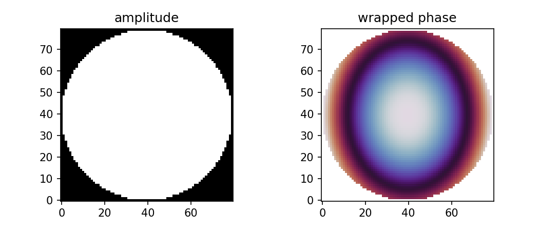
9. Visualizing OPD, phase, and amplitude

Before moving to PSF, always look at the pupil data.

A good rule is:

Never Fourier-transform a pupil function you have not inspected.

We can plot three things:

1. OPD in waves.
2. Wrapped phase.
3. Amplitude mask.

OPD in waves is:

$$\frac{W(x,y)}{\lambda}$$

This is often easier to interpret than meters.

def show_pupil_maps(opd, phase, pupil, mask, wavelength):
    opd_waves = opd / wavelength

    wrapped_phase = np.angle(pupil)

    opd_plot = np.where(mask, opd_waves, np.nan)
    phase_plot = np.where(mask, wrapped_phase, np.nan)
    amp_plot = np.abs(pupil)

    plt.figure(figsize=(5, 4))
    plt.imshow(opd_plot, origin="lower", extent=[-1, 1, -1, 1])
    plt.colorbar(label="OPD [waves]")
    plt.title("OPD map")
    plt.xlabel("Normalized pupil x")
    plt.ylabel("Normalized pupil y")
    plt.tight_layout()
    plt.show()

    plt.figure(figsize=(5, 4))
    plt.imshow(phase_plot, origin="lower", extent=[-1, 1, -1, 1])
    plt.colorbar(label="Wrapped phase [rad]")
    plt.title("Pupil phase")
    plt.xlabel("Normalized pupil x")
    plt.ylabel("Normalized pupil y")
    plt.tight_layout()
    plt.show()

    plt.figure(figsize=(5, 4))
    plt.imshow(amp_plot, origin="lower", extent=[-1, 1, -1, 1])
    plt.colorbar(label="Field amplitude")
    plt.title("Pupil amplitude")
    plt.xlabel("Normalized pupil x")
    plt.ylabel("Normalized pupil y")
    plt.tight_layout()
    plt.show()


show_pupil_maps(opd, phase, pupil, mask, wavelength)

There are a few things to notice.

The OPD map may look smooth and continuous.

The phase map may appear to jump suddenly. That does not necessarily mean the wavefront is discontinuous. It may only mean that phase is wrapped between $-\pi$ and $\pi$.

This is a common source of confusion.

The complex exponential does not care whether phase is written as:

$$0$$

or:

$$2\pi$$

Those are the same point on the unit circle.

So when you plot phase using np.angle, you are usually seeing wrapped phase. Wrapped phase is useful, but it can make smooth wavefronts look like they contain sharp jumps.

The OPD map is often better for understanding the physical wavefront. The wrapped phase map is better for checking the complex field that will go into the FFT.

10. Phase wrapping is not automatically an error

Let us pause here because this mistake is very common.

Suppose the OPD gradually increases from 0 to one wavelength across the pupil. The phase increases from:

$$0$$

to:

$$2\pi$$

But np.angle usually displays complex phase in the range:

$$-\pi \leq \phi \leq \pi$$

So when phase passes $\pi$, the plotted value jumps to $-\pi$.

That jump looks dramatic, but it may only be a display convention.

The complex number itself is continuous around the unit circle:

$$\exp(i\pi) = -1$$

and:

$$\exp(-i\pi) = -1$$

So the two edges of the displayed jump may represent nearly the same complex value.

This is why you should inspect both:

OPD in waves
wrapped phase

OPD tells you the physical wavefront error.

Wrapped phase tells you the phase as stored in the complex pupil.

They answer related but different questions.

11. A clear circular aperture with no aberration

Before using an aberrated wavefront, it helps to build the perfect case.

If OPD is zero everywhere inside the pupil:

$$W(x,y)=0$$

then:

$$P(x,y)=A(x,y)\exp(0)=A(x,y)$$

For a clear circular aperture:

$$P(x,y)=M(x,y)$$

So the pupil function is just a flat disk of complex value $1+0i$.

zero_opd = np.zeros_like(rho)

perfect_pupil, perfect_phase = pupil_function_from_opd(
    opd=zero_opd,
    mask=mask,
    wavelength=wavelength
)

print(np.max(np.abs(perfect_pupil)))
print(np.min(np.abs(perfect_pupil[mask])))

Inside the pupil, the amplitude should be 1.

Outside the pupil, the field should be 0.

This perfect pupil is the input that will produce the familiar diffraction-limited Airy pattern in the next chapter.

At this stage, we are not yet calculating the Airy pattern. We are only preparing the field that produces it.

The chain is:

flat circular pupil
→ Fourier transform
→ Airy-like PSF

Aberrations modify the pupil phase. They do not necessarily change the pupil amplitude.

So an aberrated pupil may still have amplitude 1 inside the aperture, but its phase is no longer flat.

That is the central idea:

A clear aberrated system can have uniform amplitude but non-uniform phase.

12. Adding a central obstruction

Now let us modify only the amplitude.

This example is useful because it separates two effects:

• aperture shape affects amplitude;
• OPD affects phase.

A central obstruction can be represented by blocking the middle of the pupil.

def annular_amplitude(rho, inner_radius=0.3):
    """
    Field amplitude for an annular pupil.
    """
    return ((rho >= inner_radius) & (rho <= 1.0)).astype(float)


amplitude_annular = annular_amplitude(rho, inner_radius=0.3)

annular_pupil, annular_phase = pupil_function_from_opd(
    opd=zero_opd,
    mask=mask,
    wavelength=wavelength,
    amplitude=amplitude_annular
)

Here the OPD is still zero. The phase is still flat. But the pupil amplitude has changed.

That means the PSF will change even without aberration.

This is an important lesson:

Not every PSF change comes from wavefront error.
Some PSF changes come from aperture shape and amplitude transmission.

If you model a telescope and forget the central obstruction, your diffraction pattern will be wrong even if your OPD is perfect.

If you model vignetting incorrectly, your PSF and MTF can change because the pupil amplitude changed.

Again, beautiful output is not proof of correct input.

13. What Optiland contributes at this step

Our minimal code has used a synthetic OPD map. That is useful for learning, but it is not how a real lens analysis normally begins.

In a real optical system, the OPD should come from the optical prescription:

surfaces
→ materials
→ wavelengths
→ fields
→ pupil sampling
→ ray tracing
→ reference wavefront
→ OPD map

This is where a tool such as Optiland becomes useful. The educational pattern should be:

Use Optiland or another optical design library to compute OPD from a real system.
Then use the same pupil-function formula to understand what happens next.

The exact API can change across versions, so the safest way to write this in a book project is to lock the library version in the companion code. Conceptually, the workflow looks like this:

# Version-checked workflow.
# Check the installed Optiland version and documentation
# before using exact class and method names.

# 1. Build or load an optical system.
# optic = ...

# 2. Choose field and wavelength.
# field = ...
# wavelength = 550e-9

# 3. Run wavefront / OPD analysis.
# wavefront = ...
# opd = wavefront.opd_map(...)

# 4. Get or define the pupil mask.
# mask = wavefront.pupil_mask(...)

# 5. Convert OPD to a complex pupil function.
# pupil, phase = pupil_function_from_opd(opd, mask, wavelength)

This is not meant to replace Optiland’s internal PSF tools. Instead, it explains the bridge.

If Optiland gives you an OPD map, you now know what the next mathematical step is:

$$P(x, y) = A(x, y)\exp\left(i\frac{2\pi W(x, y)}{\lambda}\right)$$

And if Optiland directly gives you a PSF, you now know one of the hidden inputs that PSF calculation depends on.

That is the point of the double-track method in this book.

The library performs the complete engineering workflow. The minimal code lets you see the calculation skeleton.

14. Sign convention: the quiet source of disagreement

There is one detail we should treat carefully: the sign in the exponential.

You may see pupil functions written as:

$$P(x,y)=A(x,y)\exp\left(i\frac{2\pi W(x,y)}{\lambda}\right)$$

or:

$$P(x,y)=A(x,y)\exp\left(-i\frac{2\pi W(x,y)}{\lambda}\right)$$

Both conventions appear in optics and signal processing contexts, often depending on the Fourier transform convention and the definition of OPD.

This is annoying, but it is manageable.

The rule is not “one sign is always correct.” The rule is:

Use a consistent sign convention across OPD, pupil function, Fourier transform, and coordinate definitions.

For intensity PSF alone, changing the sign of a real phase function often produces a related or mirrored result. But when you care about phase-sensitive quantities, asymmetric aberrations, coherent imaging, or comparing against a software package, the convention matters.

For this book’s minimal code, we will use:

$$P(x, y)=A(x,y)\exp\left(i\frac{2\pi W(x,y)}{\lambda}\right)$$

If your software package uses the opposite convention, do not panic. Check its documentation, then adapt the sign in your comparison code.

A practical comparison checklist is:

1. Use the same wavelength.
2. Use the same pupil coordinate orientation.
3. Use the same OPD reference.
4. Use the same phase sign convention.
5. Use the same FFT convention when moving to PSF.

When two programs disagree, the first suspect should not be “the physics is wrong.” The first suspects should be units, signs, sampling, and normalization.

15. Pupil coordinates: physical or normalized?

In this chapter we used normalized coordinates:

$$-1 \leq x \leq 1$$

$$-1 \leq y \leq 1$$

with the circular pupil defined by:

$$x^2+y^2 \leq 1$$

This is convenient for teaching.

In a real optical system, pupil coordinates may also be expressed in physical units, such as millimeters. A pupil radius might be:

$$R_\text{pupil}=5\text{ mm}$$

Then a physical pupil coordinate $(X,Y)$ can be normalized as:

$$x = \frac{X}{R_\text{pupil}}$$

$$y = \frac{Y}{R_\text{pupil}}$$

The OPD itself is not automatically normalized. OPD remains a length.

So you might have:

x, y: normalized pupil coordinates
W: meters
λ: meters
phase: radians

That combination is perfectly fine.

The coordinate system describes where you are in the pupil. OPD and wavelength describe how much phase delay exists there.

Keep these roles separate:

pupil coordinate: position
OPD: path difference
wavelength: scale for phase conversion
phase: angle in radians

When this separation is clear, the code becomes much easier to debug.

16. The pupil function is not the PSF

This is worth saying plainly.

The pupil function is not the image of a point source.

The pupil function lives in the pupil plane. It describes the complex field across the aperture.

The PSF lives in the image plane. It describes intensity distribution after diffraction and aberration.

The next chapter will connect them through a Fourier transform, but they are not the same object.

A rough map is:

Pupil plane:
complex field over aperture

Image plane:
intensity distribution around image point

This matters because a phase map can look severe while the resulting PSF may still be compact, or a small-looking pupil obstruction can produce visible diffraction rings.

You cannot always read the final image quality directly from one pupil plot. The pupil function is the input. The PSF is the output after coherent propagation.

That is why we are building the chain carefully instead of jumping straight to the final plot.

17. A complete minimal script

Here is a compact version of the whole chapter’s minimal implementation.

It creates:

• a pupil grid;
• a circular mask;
• a synthetic OPD map;
• a complex pupil function;
• plots for OPD, phase, and amplitude.

import numpy as np
import matplotlib.pyplot as plt


def make_pupil_grid(n=256):
    coord = np.linspace(-1.0, 1.0, n)
    x, y = np.meshgrid(coord, coord)

    rho = np.sqrt(x**2 + y**2)
    theta = np.arctan2(y, x)
    mask = rho <= 1.0

    return x, y, rho, theta, mask


def synthetic_opd(rho, theta, mask, wavelength):
    opd = np.zeros_like(rho)

    defocus = 0.50 * wavelength
    astigmatism = 0.25 * wavelength

    opd += defocus * (2.0 * rho**2 - 1.0)
    opd += astigmatism * rho**2 * np.cos(2.0 * theta)

    opd[~mask] = 0.0

    return opd


def pupil_function_from_opd(opd, mask, wavelength, amplitude=None):
    if amplitude is None:
        amplitude = mask.astype(float)

    phase = 2.0 * np.pi * opd / wavelength
    pupil = amplitude * np.exp(1j * phase)

    pupil[~mask] = 0.0 + 0.0j

    return pupil, phase


def plot_map(data, title, colorbar_label):
    plt.figure(figsize=(5, 4))
    plt.imshow(data, origin="lower", extent=[-1, 1, -1, 1])
    plt.colorbar(label=colorbar_label)
    plt.title(title)
    plt.xlabel("Normalized pupil x")
    plt.ylabel("Normalized pupil y")
    plt.tight_layout()
    plt.show()


wavelength = 550e-9

x, y, rho, theta, mask = make_pupil_grid(n=256)
opd = synthetic_opd(rho, theta, mask, wavelength)

pupil, phase = pupil_function_from_opd(
    opd=opd,
    mask=mask,
    wavelength=wavelength
)

opd_waves = np.where(mask, opd / wavelength, np.nan)
wrapped_phase = np.where(mask, np.angle(pupil), np.nan)
amplitude = np.abs(pupil)

plot_map(opd_waves, "OPD map", "OPD [waves]")
plot_map(wrapped_phase, "Wrapped pupil phase", "Phase [rad]")
plot_map(amplitude, "Pupil amplitude", "Field amplitude")

This script does not yet calculate the PSF. That is deliberate.

At this point, the correct question is not:

Where is the image?

The correct question is:

Have we correctly built the complex field that will form the image?

Once that answer is yes, the Fourier transform in the next chapter will make sense.

18. Common mistakes

Let us collect the most common errors before moving on.

Mistake 1: Mixing units

This is the most dangerous one.

Wrong:

opd = 200      # nanometers, but not labeled
wavelength = 550e-9  # meters
phase = 2 * np.pi * opd / wavelength

Correct:

opd = 200e-9
wavelength = 550e-9
phase = 2 * np.pi * opd / wavelength

Always make OPD and wavelength use the same unit.

Mistake 2: Forgetting the aperture mask

If you compute:

pupil = np.exp(1j * phase)

without applying the mask, you have allowed light through the whole square array.

Correct:

pupil = mask.astype(float) * np.exp(1j * phase)
pupil[~mask] = 0.0

The FFT does not know your aperture is supposed to be circular unless you tell it.

Mistake 3: Confusing amplitude and intensity

If a filter transmits 25% of intensity, the field amplitude factor is not 0.25. It is:

$$\sqrt{0.25}=0.5$$

Wrong:

amplitude = intensity_transmission

Usually correct:

amplitude = np.sqrt(intensity_transmission)

This matters because PSF intensity is calculated from the squared magnitude of a complex field.

Mistake 4: Thinking wrapped phase jumps are always physical jumps

A sudden jump in np.angle(pupil) may only be phase wrapping.

Check OPD in waves before deciding the wavefront is discontinuous.

Mistake 5: Comparing against software without checking conventions

If your PSF differs from a software package, check:

• wavelength;
• pupil sampling;
• OPD reference;
• phase sign;
• FFT shift;
• normalization;
• coordinate orientation.

Do this before changing the physics.

Mistake 6: Treating the pupil function as a final result

The pupil function is an intermediate representation. It is extremely important, but it is not the PSF and not the MTF.

Its job is to carry amplitude and phase information into the diffraction calculation.

19. What this chapter adds to the full chain

We can now update the book’s main computation chain:

lens prescription
→ surfaces and materials
→ ray tracing
→ optical path length
→ OPD map
→ pupil amplitude
→ pupil phase
→ complex pupil function

This chapter performed one precise conversion:

OPD in length units
→ phase in radians
→ complex field over the aperture

That conversion is small enough to fit in a few lines of code. But conceptually, it is one of the most important steps in the book.

Without it, OPD remains only a wavefront error map.

With it, the wavefront becomes something that can interfere, diffract, and form an image.

That is why the pupil function is the doorway into PSF calculation.

In the next chapter, we will send this complex pupil function through a Fourier transform. The result will no longer live in the pupil plane. It will become the intensity distribution of a point image: the PSF.

And from that PSF, we will finally be close to the MTF curve that started this whole journey.

Chapter summary

The pupil function stores the complex field across the aperture.

It combines:

amplitude
phase
aperture mask

The central formula is:

$$P(x, y) = A(x, y)\exp\left(i\frac{2\pi W(x, y)}{\lambda}\right)$$

where OPD $W(x,y)$ must use the same length unit as wavelength $\lambda$.

The aperture mask tells the code where light exists. The amplitude tells how much field passes through. The phase tells how OPD changes the complex field.

A perfect clear circular pupil has flat phase and uniform amplitude. An aberrated pupil may have uniform amplitude but non-uniform phase. An obstructed or apodized pupil may have non-uniform amplitude even with zero OPD.

The main code action in this chapter was:

phase = 2.0 * np.pi * opd / wavelength
pupil = amplitude * np.exp(1j * phase)
pupil[~mask] = 0.0

That is the bridge from OPD to Fourier optics.

Next, we will use this pupil function to compute the PSF.

Generated validation figure