Chapter 10: OPD and Wavefront Error
A spot diagram tells us where rays land.
That is useful. Very useful. In Chapter 7, the spot diagram was our first real analysis plot. In Chapter 9, ray fans helped us see how real rays depart from a paraxial reference. We could look at transverse ray error and begin to recognize spherical aberration, coma, astigmatism, field curvature, distortion, and chromatic effects.
But there is a limit to this way of looking.
A ray can land near the right place and still arrive with the wrong phase.
That sentence is the doorway to the next part of the book.
Geometric ray tracing tracks where rays go. Diffraction imaging cares about how the optical field adds up. To compute a PSF by Fourier methods, we need not only a collection of ray intercepts. We need a complex pupil function. To build that pupil function, we need phase across the pupil. To get phase, we need optical path difference.
That is the bridge:
real ray tracing
→ optical path length
→ optical path difference
→ wavefront error
→ pupil phase
→ PSF
→ OTF
→ MTF
This chapter is about the middle of that bridge.
We will ask:
What is optical path length?
What is OPD?
What is the reference wavefront?
Why is OPD usually shown over the pupil?
How can we create a simple OPD map in Python?
How does this connect to Optiland wavefront analysis?
We will not compute a production-quality OPD from a full ray trace in this chapter. That requires careful reference geometry, exit pupil coordinates, ray aiming, focus conventions, and surface-by-surface optical path bookkeeping. A real library handles those details. Current Optiland wavefront tools, for example, include OPD and wavefront analysis modules, and its Wavefront class is documented as computing exit-pupil ray intersections, OPD, ray intensities, and reference-sphere radius according to selected strategies. (Optiland)
Our job here is to understand what those tools are calculating.
So we will do two things:
1. Build the concept carefully.
2. Generate simplified OPD maps ourselves.
Once you understand the OPD map, Chapter 11 can turn it into a complex pupil function.
That is the moment geometric optics becomes Fourier optics.
Why ray landing points are not enough
Imagine two rays that reach the same point on the image plane.
From a spot diagram alone, they look perfect. They landed together.
But suppose one ray has traveled a slightly longer optical path than the other. Then their phases may not match when the waves interfere. If the phase difference is small, they add mostly constructively. If the phase difference is large, they may partially cancel or create structure in the diffraction pattern.
A spot diagram cannot show that.
A spot diagram records transverse position:
x_image, y_image
A wavefront analysis records optical path difference across the pupil:
OPD(Px, Py)
These are different kinds of data.
Ray intercepts answer:
Where did the rays go?
OPD answers:
How much optical phase delay does each pupil point carry relative to a reference?
Both matter.
For a badly aberrated lens, spot diagrams can be very informative. For a nearly diffraction-limited lens, spot diagrams may become less revealing. The geometric spot may be tiny, but the wavefront phase still determines the detailed diffraction pattern.
That is why we need OPD.
It is the missing quantity between ray tracing and PSF.
Optical path length
A ray traveling through air and glass does not only cover geometric distance. It accumulates optical path length.
For a small segment of length ds in a medium of refractive index n, the optical path contribution is:
dOPL = n ds
Along a full path:
OPL = ∫ n ds
In a ray tracer with discrete segments, this becomes:
OPL = n1 s1 + n2 s2 + n3 s3 + ...
where:
s1, s2, s3 = geometric segment lengths
n1, n2, n3 = refractive indices along those segments
This is why our Ray class has carried opl since Chapter 4.
When we wrote:
ray.propagate(distance, refractive_index=n)
we updated:
ray.opl += n * distance
At the time, that may have looked like extra bookkeeping. Now it becomes essential.
The ray’s final position tells us where it landed.
The ray’s accumulated OPL tells us how much optical distance it traveled.
Those two pieces of information lead to different analyses.
A tiny OPL example
Let us revisit the simplest possible path.
A ray travels:
20 mm in air
5 mm in glass
20 mm in air
If the glass index is 1.5, then:
geometric distance = 20 + 5 + 20 = 45 mm
OPL = 1.0×20 + 1.5×5 + 1.0×20 = 47.5 mm
In code:
segments = [
    {"distance_mm": 20.0, "n": 1.0},
    {"distance_mm": 5.0,  "n": 1.5},
    {"distance_mm": 20.0, "n": 1.0},
]

opl = sum(seg["distance_mm"] * seg["n"] for seg in segments)
geometric = sum(seg["distance_mm"] for seg in segments)

print("geometric distance [mm]:", geometric)
print("optical path length [mm]:", opl)
The ray has physically traveled 45 mm, but optically it has traveled 47.5 mm.
This difference is not cosmetic. It determines phase.
If another ray travels a slightly different optical path, the two rays may arrive with different phase even if their geometric endpoints are close.
From OPL to OPD
Optical path length by itself is not yet wavefront error.
OPL is an absolute accumulated path along one ray. OPD is a difference relative to a reference.
A simple definition is:
OPD = OPL_ray - OPL_reference
But the reference matters.
For imaging, the ideal reference is usually not a flat plane. A perfect converging wave heading toward an image point has a spherical wavefront centered on that image point. So the reference wavefront is often a sphere.
That means OPD is more carefully understood as:
the optical path difference between the actual wavefront and a chosen reference wavefront
or, in ray terms:
how much each ray's optical path differs from the ideal reference path
This is where wavefront analysis becomes a little subtle. We must decide what “ideal” means.
Possible reference choices include:
chief-ray reference sphere
centroid-based reference sphere
best-fit reference sphere
paraxial reference sphere
image-plane reference
Different choices remove or retain different low-order terms such as piston, tilt, and defocus. This is not cheating. It is choosing what question the OPD map should answer.
Current Optiland documentation reflects this idea directly: its Wavefront analysis accepts strategy choices such as chief_ray, centroid_sphere, and best_fit_sphere, and includes a remove_tilt option for OPD data. (Optiland)
That tells us something important:
OPD is not only a raw number. It is a number relative to a reference geometry.
The reference must be known before the OPD map can be interpreted.
OPD in length and OPD in waves
OPD can be expressed in length units:
OPD = 0.00025 mm
It can also be expressed in waves:
OPD_waves = OPD_length / wavelength
This is often more useful for phase.
If the wavelength is 0.5 µm, then an OPD of 0.25 µm is half a wave:
0.25 µm / 0.5 µm = 0.5 waves
Phase is related to OPD in waves by:
phase = 2π × OPD_waves
or, using length units:
phase = 2π × OPD_length / wavelength
This unit conversion is a place where mistakes love to hide.
If OPL is stored in millimeters and wavelength is stored in micrometers, we must convert:
wavelength_mm = wavelength_um × 1e-3
Then:
OPD_waves = OPD_mm / wavelength_mm
Let us write helpers:
import numpy as np
import math
import matplotlib.pyplot as plt

def wavelength_um_to_mm(wavelength_um):
    return wavelength_um * 1e-3

def opd_mm_to_waves(opd_mm, wavelength_um):
    wavelength_mm = wavelength_um_to_mm(wavelength_um)
    return opd_mm / wavelength_mm

def opd_waves_to_phase(opd_waves):
    return 2.0 * np.pi * opd_waves
Test:
opd_um = 0.25
wavelength_um = 0.5

opd_mm = opd_um * 1e-3
waves = opd_mm_to_waves(opd_mm, wavelength_um)

print("OPD [waves]:", waves)
print("phase [radians]:", opd_waves_to_phase(waves))
The result should be:
0.5 waves
π radians
This is the step that Chapter 11 will use directly.
Pupil coordinates
OPD is usually shown as a function over the pupil.
Instead of plotting OPD versus image-plane coordinates, we plot it over normalized pupil coordinates:
Px, Py
where the pupil circle is:
Px² + Py² <= 1
A pupil coordinate identifies where a sampled ray passes through the pupil. For each point in the pupil, the wavefront has some optical path difference relative to the reference.
So an OPD map is:
OPD(Px, Py)
This is why wavefront maps look like colored disks. The disk is the pupil. The color is OPD.
Let us create a pupil grid.
def make_normalized_pupil_grid(N):
    """Create a square grid with a circular pupil mask.

    Returns
    -------
    X, Y:
        Meshgrid coordinates from -1 to +1.

    R:
        Radius sqrt(X^2 + Y^2).

    mask:
        Boolean circular aperture mask.
    """
    u = np.linspace(-1.0, 1.0, N)
    X, Y = np.meshgrid(u, u)
    R = np.sqrt(X**2 + Y**2)
    mask = R <= 1.0
    return X, Y, R, mask
Plot the mask:
X, Y, R, mask = make_normalized_pupil_grid(256)

plt.imshow(mask, extent=[-1, 1, -1, 1], origin="lower")
plt.xlabel("Pupil X")
plt.ylabel("Pupil Y")
plt.title("Circular pupil mask")
plt.colorbar(label="inside pupil")
plt.show()
This is not yet OPD. It is the domain where OPD will live.
A simplified wavefront function
Now we will generate an OPD map directly.
This is not yet computed from a full ray trace. It is a controlled teaching model. We choose a wavefront error function over the pupil, then visualize it.
This is useful because the goal of this chapter is representation:
OPD over pupil → phase → pupil function
The source of the OPD can be a real ray trace, a fitted Zernike model, a measured wavefront sensor, or a simplified polynomial. The representation is the same.
Let us build a toy wavefront in waves.
Use normalized pupil coordinates:
X, Y ∈ [-1, 1]
R² = X² + Y²
Add simple terms:
defocus-like term:      2R² - 1
astigmatism-like term:  X² - Y²
coma-like term:         (3R² - 2)Y
spherical-like term:    6R⁴ - 6R² + 1
These are not carefully normalized Zernike polynomials. They are teaching shapes. That is enough for seeing how OPD maps work.
def toy_opd_waves(X, Y, mask, defocus=0.0, astig=0.0, coma=0.0, spherical=0.0):
    """Create a toy OPD map in waves over a normalized circular pupil.

    The terms are simple teaching polynomials, not normalized Zernikes.
    """
    R2 = X**2 + Y**2
    R4 = R2**2

    W = np.zeros_like(X, dtype=float)

    W += defocus * (2.0 * R2 - 1.0)
    W += astig * (X**2 - Y**2)
    W += coma * (3.0 * R2 - 2.0) * Y
    W += spherical * (6.0 * R4 - 6.0 * R2 + 1.0)

    W = np.where(mask, W, np.nan)
    return W
Now create a map:
X, Y, R, mask = make_normalized_pupil_grid(256)

W = toy_opd_waves(
    X, Y, mask,
    defocus=0.25,
    astig=0.10,
    coma=0.08,
    spherical=0.05,
)
Here W is OPD in waves.
That means:
W = 1.0 means one wavelength of OPD
W = 0.5 means half a wavelength
W = 0.0 means equal to the reference
Plot it:
def plot_opd_map(W, title="OPD map [waves]"):
    plt.imshow(W, extent=[-1, 1, -1, 1], origin="lower")
    plt.xlabel("Pupil X")
    plt.ylabel("Pupil Y")
    plt.title(title)
    plt.colorbar(label="OPD [waves]")
    plt.gca().set_aspect("equal", adjustable="box")
    plt.show()

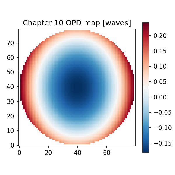
plot_opd_map(W, title="Toy OPD map")
Now we have an OPD map.
It is not a spot diagram. It is not an image. It is not a PSF.
It is the wavefront error across the pupil.
Reading the OPD map
An OPD map is a height map in optical path.
High and low regions mean different parts of the pupil have different phase delays relative to the reference.
A perfectly corrected wavefront would be flat after removing irrelevant piston and tilt:
OPD(Px, Py) ≈ 0
A defocused wavefront has a bowl-like or dome-like shape.
Astigmatism changes sign along orthogonal pupil directions.
Coma has an asymmetric shape tied to field direction.
Spherical aberration is radially symmetric but changes with pupil radius in a higher-order way.
Again, do not over-memorize the pictures. The computational meaning is more important:
Each pupil point has a phase delay.
The OPD map stores that delay.
The pupil function will convert that delay into a complex phase factor.
The OPD map is not the final image-quality metric. It is an intermediate representation.
But it is the representation that lets diffraction enter.
Piston, tilt, and defocus
Some OPD terms shift the wavefront in ways that may or may not matter for a given analysis.
Piston
Piston is a constant OPD added everywhere:
W_new(Px, Py) = W(Px, Py) + constant
This adds the same phase to the whole pupil. For intensity PSF, a global phase factor usually does not change the result. So piston is often removed.
Tilt
Tilt is a linear phase ramp across the pupil:
W(Px, Py) = a Px + b Py
Tilt shifts the PSF position. If you want to analyze image quality independent of pointing or chief-ray shift, you may remove tilt. If you care about image displacement, you may keep it.
Defocus
Defocus is a quadratic wavefront term. Removing defocus corresponds to changing the reference focus. Sometimes you want to remove it to evaluate best focus. Sometimes you want to keep it to see how far the current image plane is from focus.
This is why wavefront software often offers options for removing or retaining low-order terms.
A map with piston removed is not “more true.” It answers a different question.
Let us write a simple piston removal:
def remove_piston(W, mask):
    """Subtract mean OPD over the pupil."""
    W2 = W.copy()
    mean = np.nanmean(W2[mask])
    W2[mask] -= mean
    return W2
Use it:
W_no_piston = remove_piston(W, mask)

print("mean before:", np.nanmean(W[mask]))
print("mean after:", np.nanmean(W_no_piston[mask]))
For tilt removal, fit a plane:
def remove_piston_and_tilt(W, X, Y, mask):
    """Remove best-fit plane a + bX + cY from W over the pupil."""
    valid = mask & np.isfinite(W)

    A = np.column_stack([
        np.ones(np.count_nonzero(valid)),
        X[valid],
        Y[valid],
    ])

    b = W[valid]
    coeffs, *_ = np.linalg.lstsq(A, b, rcond=None)

    plane = coeffs[0] + coeffs[1] * X + coeffs[2] * Y
    W2 = W.copy()
    W2[valid] = W[valid] - plane[valid]

    return W2, coeffs
Use it:
W_flat, coeffs = remove_piston_and_tilt(W, X, Y, mask)

print("removed plane coefficients:", coeffs)
plot_opd_map(W_flat, title="Toy OPD map after piston and tilt removal")
This code is intentionally simple. A real optical wavefront tool may use reference spheres, ray aiming, Zernike fitting, or best-fit strategies. But the idea is the same:
remove terms that represent reference choice
inspect the residual wavefront error
RMS and peak-to-valley wavefront error
Two common OPD summaries are RMS wavefront error and peak-to-valley wavefront error.
RMS wavefront error is:
RMS = sqrt(mean((W - mean(W))²))
over the pupil.
Peak-to-valley is:
PV = max(W) - min(W)
over the pupil.
In code:
def wavefront_rms(W, mask):
    valid = mask & np.isfinite(W)
    values = W[valid]
    values = values - np.mean(values)
    return math.sqrt(float(np.mean(values**2)))

def wavefront_pv(W, mask):
    valid = mask & np.isfinite(W)
    values = W[valid]
    return float(np.max(values) - np.min(values))
Compute:
print("RMS [waves]:", wavefront_rms(W, mask))
print("PV [waves]:", wavefront_pv(W, mask))
These numbers are useful, but they are not the whole story.
A wavefront with the same RMS can have different spatial structure. One may be mostly defocus. Another may have high-frequency ripple. Their PSFs may differ. Their MTFs may differ.
So RMS is a summary, not an image-quality oracle.
This lesson should now feel familiar. Spot RMS did not replace spot diagrams. Wavefront RMS does not replace the OPD map or PSF.
OPD in millimeters, micrometers, and waves
Let us convert our toy wavefront from waves to physical length.
Suppose wavelength is:
λ = 0.5876 µm
Then:
OPD_um = W_waves × λ_um
and:
OPD_mm = OPD_um × 1e-3
In code:
def opd_waves_to_um(W_waves, wavelength_um):
    return W_waves * wavelength_um

def opd_waves_to_mm(W_waves, wavelength_um):
    return W_waves * wavelength_um * 1e-3
Example:
wavelength_um = 0.5876

W_rms_waves = wavefront_rms(W, mask)
W_rms_um = opd_waves_to_um(W_rms_waves, wavelength_um)

print("RMS [waves]:", W_rms_waves)
print("RMS [µm]:", W_rms_um)
This conversion matters because different tools report OPD differently. Some report waves. Some report length. Some label plots in nanometers. Some normalize by the analysis wavelength.
Optiland’s WavefrontData documentation, for example, describes the opd field as optical path difference data normalized to waves. (Optiland)
So if you compare outputs between tools, always check the unit.
A wavefront error of 0.1 waves at 0.5 µm is not the same physical length as 0.1 waves at 10 µm.
In waves, they look equal. In micrometers, they are not.
A line profile: OPD fan
An OPD map is a two-dimensional pupil plot.
An OPD fan is the wavefront version of a ray fan: it shows OPD along a line through the pupil.
For example:
OPD(Px, 0)
or:
OPD(0, Py)
Let us extract a horizontal line through the center.
def center_line_profile(W, axis="x"):
    N = W.shape[0]
    c = N // 2

    if axis == "x":
        coord = np.linspace(-1.0, 1.0, N)
        values = W[c, :]
    elif axis == "y":
        coord = np.linspace(-1.0, 1.0, N)
        values = W[:, c]
    else:
        raise ValueError("axis must be 'x' or 'y'")

    return coord, values
Plot:
px, wx = center_line_profile(W_no_piston, axis="x")

plt.plot(px, wx)
plt.axhline(0.0, linewidth=0.8)
plt.axvline(0.0, linewidth=0.8)
plt.xlabel("Pupil X")
plt.ylabel("OPD [waves]")
plt.title("OPD fan through pupil center")
plt.show()
This looks similar in spirit to a ray fan, but the vertical axis is different.
Ray fan:
transverse image error [mm]
OPD fan:
optical path difference [waves or length]
Both are pupil-coordinate diagnostics. They answer different questions.
Ray aberration and wave aberration are related but not identical
It is tempting to say:
ray fan is the slope of the wavefront
There is truth in that idea, but it deserves care. In classical optical theory, transverse ray aberrations are related to derivatives of wave aberration under certain approximations. At high numerical aperture or with complex wavefront structure, the relationship can require more careful treatment.
For this book, the practical message is:
Ray fans show where rays miss in the image plane.
OPD maps show optical path error across the pupil.
They are connected, but one is not a simple replacement for the other in every regime.
This is enough for our computation chain.
We do not need to derive the full mathematical relation here. We need to understand why the next representation is necessary.
Ray landing positions led us to spot diagrams and ray fans.
Optical path differences lead us to pupil phase and diffraction.
That is the transition.
From OPD to phase
Now comes the most important line in the chapter.
If W is OPD in waves, then the pupil phase is:
φ(Px, Py) = 2π W(Px, Py)
In code:
phase = 2.0 * np.pi * W_no_piston
If OPD is in millimeters, then:
phase = 2.0 * np.pi * opd_mm / wavelength_mm
This phase is what the complex pupil function uses:
P(Px, Py) = A(Px, Py) exp(i φ(Px, Py))
where:
A(Px, Py) = aperture amplitude
φ(Px, Py) = phase from OPD
Do not rush through this. It is the handoff between Chapter 10 and Chapter 11.
The OPD map is real-valued.
The pupil function is complex-valued.
The conversion is through phase.
That is how wavefront error becomes something Fourier optics can use.
A preview of the pupil phase
Let us plot phase wrapped between -π and π.
def wrap_phase(phase):
    """Wrap phase to [-pi, pi]."""
    return (phase + np.pi) % (2.0 * np.pi) - np.pi

phase = opd_waves_to_phase(W_no_piston)
phase_wrapped = np.where(mask, wrap_phase(phase), np.nan)

plt.imshow(phase_wrapped, extent=[-1, 1, -1, 1], origin="lower")
plt.xlabel("Pupil X")
plt.ylabel("Pupil Y")
plt.title("Wrapped pupil phase")
plt.colorbar(label="phase [radians]")
plt.gca().set_aspect("equal", adjustable="box")
plt.show()
This plot may look more abrupt than the OPD map because phase wrapping jumps at ±π. That does not mean the wavefront physically jumps there. It means the phase display is wrapped modulo 2π.
This is another common source of confusion.
OPD is often easier to read for smooth wavefront error.
Wrapped phase is useful for seeing the complex field’s periodic nature.
Both are views of the same underlying delay.
A deliberately simple OPD-to-PSF preview
We are not doing the full PSF chapter yet, but a tiny preview helps show why OPD matters.
Given:
aperture amplitude A
phase φ
the pupil field is:
pupil = A exp(iφ)
A simplified Fraunhofer PSF can be computed from the squared magnitude of the Fourier transform of the pupil field.
Do not worry about scaling yet. Chapter 12 will handle this properly. Here, the purpose is only to show that changing OPD changes the diffraction pattern.
def quick_psf_from_opd(W_waves, mask):
    """A minimal, unscaled PSF preview from OPD in waves.

    This is for intuition only. Chapter 12 will handle sampling and scaling.
    """
    phase = 2.0 * np.pi * np.nan_to_num(W_waves, nan=0.0)
    pupil = mask.astype(float) * np.exp(1j * phase)

    field = np.fft.fftshift(np.fft.fft2(np.fft.ifftshift(pupil)))
    psf = np.abs(field)**2
    psf = psf / psf.sum()

    return psf
Compare a flat wavefront and an aberrated one:
W_flat = np.where(mask, 0.0, np.nan)
psf_flat = quick_psf_from_opd(W_flat, mask)
psf_aberrated = quick_psf_from_opd(W_no_piston, mask)
Plot one:
def plot_psf_preview(psf, title):
    plt.imshow(np.log10(psf + 1e-12), origin="lower")
    plt.title(title)
    plt.colorbar(label="log10 intensity")
    plt.show()

plot_psf_preview(psf_flat, "Preview PSF: flat wavefront")
plot_psf_preview(psf_aberrated, "Preview PSF: aberrated wavefront")
This is only a preview, but it makes the bridge visible.
The spot diagram came from ray intercepts.
The PSF comes from a complex pupil field.
The complex pupil field comes from aperture amplitude and OPD-derived phase.
So PSF/MTF cannot be fully explained by ray landing points alone.
They need wavefront phase.
How real ray tracing would provide OPD
Our toy OPD map was created from polynomial terms. A real wavefront analysis must compute OPD from the optical system.
Conceptually, the steps look like this:
1. Choose field and wavelength.
2. Sample rays across the pupil.
3. Trace rays through the optical system.
4. Accumulate optical path length for each ray.
5. Determine a reference wavefront or reference sphere.
6. Compare each ray's optical path to the reference.
7. Store OPD over pupil coordinates.
8. Optionally remove piston, tilt, or focus terms.
Step 5 is the delicate one. The reference wavefront is what makes OPD meaningful. Without it, you only have OPL values, not wavefront error.
This is also why production tools expose strategy options. The strategy defines how the reference geometry is chosen.
In Optiland’s documented Wavefront class, the parameters include fields, wavelengths, number of rays, distribution pattern such as hexapolar, strategy choice, afocal mode, and tilt removal. The documentation states that the class computes exit-pupil ray intersections, OPD, ray intensities, and reference sphere radius. (Optiland)
That is the library-level version of the conceptual list above.
A simplified OPD-from-OPL sketch
Let us write a sketch to clarify the difference between OPL and OPD.
Suppose we have several rays, each with:
pupil coordinate
OPL
reference OPL
Then:
def compute_opd_from_opl(opl_values, reference_opl_values):
    """Compute OPD as OPL difference."""
    return np.asarray(opl_values) - np.asarray(reference_opl_values)
If the reference is just the chief ray OPL, then:
def compute_opd_relative_to_chief(opl_values, chief_index):
    opl_values = np.asarray(opl_values, dtype=float)
    return opl_values - opl_values[chief_index]
This is simple, but it is not a full imaging OPD calculation. A chief-ray OPL difference alone may not include the correct spherical reference to the image point. It may mix in tilt or defocus depending on geometry.
That is why this code is only a sketch.
The real point is:
OPL is accumulated along rays.
OPD is OPL compared with a chosen reference.
Wavefront error is OPD interpreted over the pupil.
Keep those three separate.
Optiland OPD map comparison
Optiland provides higher-level OPD tools, so a real workflow can be much shorter than our teaching model.
The current documentation gallery shows an OPD map example using:
from optiland.samples.infrared import InfraredTripletF4
from optiland.wavefront import OPD

lens = InfraredTripletF4()
lens.draw()

opd = OPD(lens, field=(0, 1), wavelength=4.2)
opd.view()
The example labels the output as an OPD map over pupil coordinates and reports RMS in waves. (Optiland)
For a visible singlet, a conceptual workflow would look similar:
from optiland import optic
from optiland.wavefront import OPD

lens = optic.Optic()

lens.surfaces.add(index=0, radius=float("inf"), thickness=float("inf"))
lens.surfaces.add(index=1, radius=50.0, thickness=5.0, material="N-BK7", is_stop=True)
lens.surfaces.add(index=2, radius=-50.0, thickness=45.0)
lens.surfaces.add(index=3)

lens.set_aperture(aperture_type="EPD", value=10.0)
lens.fields.set_type("angle")
lens.fields.add(y=0.0)
lens.wavelengths.add(value=0.5876, is_primary=True)

opd = OPD(lens, field=(0, 0), wavelength=0.5876)
opd.view()
Treat this as library-level comparison code. Exact behavior may depend on the installed Optiland version and the optical model. The important computational meaning is stable:
the library samples the pupil
traces rays
computes OPD relative to reference geometry
displays OPD over pupil coordinates
The teaching code in this chapter generated OPD directly as a polynomial map. Optiland computes OPD from the actual optical system.
Both produce the same kind of object:
OPD(Px, Py)
That object is what Chapter 11 needs.
Wavefront analysis and Zernike coefficients
OPD maps are often decomposed into Zernike polynomials.
Zernikes are a set of functions over the unit disk. They are useful because the pupil is often circular, and common aberration-like shapes can be represented with low-order Zernike terms.
For example, Zernike-like terms can represent:
piston
tilt
defocus
astigmatism
coma
spherical aberration
This is why optical software often reports Zernike coefficients alongside an OPD map.
We will not derive Zernike polynomials here. The purpose of this chapter is more basic: understand the OPD map itself.
But it helps to know where Zernikes fit:
OPD map:
    raw or computed wavefront error over the pupil

Zernike fit:
    compact coefficient representation of that OPD map
A Zernike table is not a replacement for understanding OPD. It is a compact way to describe it.
Optiland’s wavefront API overview includes Zernike-related OPD modules alongside OPD, wavefront, reference geometry, and PSF/MTF modules. (Optiland)
That placement is sensible: Zernikes are part of wavefront analysis, not a separate universe.
What OPD can and cannot tell you
OPD is powerful, but we should not oversell it.
OPD can tell you:
phase error across the pupil
RMS wavefront error
peak-to-valley wavefront error
dominant low-order wavefront shapes
whether the pupil phase is nearly flat
how wavefront error differs by field or wavelength
OPD by itself does not directly tell you:
the full PSF intensity distribution
the MTF curve
sensor sampling effects
stray light
coating ghosts
manufacturing tolerances
polarization effects
scattering
OPD is an input to diffraction calculation, not the final answer.
This is the same pattern we have seen before.
The prescription is not the ray trace.
The ray trace is not the spot diagram.
The spot diagram is not the wavefront.
The wavefront is not the PSF.
The PSF is not the MTF.
Each representation keeps some information, transforms some information, and discards or summarizes some information.
The skill is knowing which representation answers which question.
A useful mental model
Here is the simplest way to remember the transition:
ray position error:
    "Where did the ray land?"

wavefront error:
    "How late or early is the wave at this pupil point?"
A ray fan plots the first kind of error against pupil coordinate.
An OPD fan plots the second kind of error against pupil coordinate.
A spot diagram shows ray landing points.
An OPD map shows phase delay across the pupil.
The PSF will show what happens when all those pupil contributions interfere.
That last word matters: interfere.
Ray diagrams do not interfere. Waves do.
OPD is how the ray-tracing world hands phase information to the wave-optics world.
Common mistakes with OPD
Let us name the traps before moving on.
Mistake 1: Confusing OPL and OPD
OPL is accumulated optical path length along a ray.
OPD is the difference between that path and a reference.
A list of OPL values is not automatically a wavefront map.
Mistake 2: Forgetting the reference geometry
OPD always depends on a reference. Chief-ray sphere, centroid sphere, best-fit sphere, paraxial focus, and image plane references can give different maps.
Ask what reference was used.
Mistake 3: Mixing length units and waves
If OPD is in millimeters and wavelength is in micrometers, convert before dividing.
wavelength_mm = wavelength_um × 1e-3
Mistake 4: Treating piston as image degradation
A constant phase offset usually does not change the intensity PSF. Piston may matter in interferometry or segmented systems, but for ordinary single-pupil PSF intensity it is often removed.
Mistake 5: Removing tilt without knowing what it means
Removing tilt recenters the wavefront phase and often shifts the PSF reference. That may be desirable, but it changes the question being asked.
Mistake 6: Treating defocus as always bad or always removable
Defocus may represent a wrong image plane, an intentional focus shift, or a term you want to optimize away. Do not remove it blindly.
Mistake 7: Reading wrapped phase as physical discontinuity
Phase wraps at ±π. A jump in wrapped phase may simply be display wrapping, not a physical discontinuity.
Mistake 8: Believing RMS wavefront error tells the whole story
RMS is useful, but different OPD shapes with the same RMS can produce different PSFs and MTFs.
Mistake 9: Forgetting wavelength dependence
The same physical OPD length corresponds to different numbers of waves at different wavelengths.
Mistake 10: Expecting OPD to replace ray plots
OPD is a wavefront representation. Ray fans and spot diagrams remain useful geometric diagnostics.
What this chapter gives us
We have now crossed the bridge from geometric ray tracing toward wave optics.
We can explain:
OPL as accumulated n ds
OPD as optical path difference relative to a reference
why OPD is plotted over pupil coordinates
why OPD can be expressed in length or waves
how OPD becomes phase
why piston, tilt, and defocus depend on analysis convention
how to generate a toy OPD map
how to compute RMS and PV wavefront error
how OPD maps differ from spot diagrams and ray fans
how Optiland's wavefront tools fit into the same chain
The core transformation is:
OPD(Px, Py) in waves
→ phase φ(Px, Py) = 2π OPD(Px, Py)
That is the exact handoff to the next chapter.
The road ahead
Now we have a real-valued wavefront error map.
But diffraction calculation needs a complex field over the pupil.
That field has two parts:
amplitude: where light passes and how strongly
phase: how much optical delay each pupil point carries
The aperture mask gives amplitude.
The OPD map gives phase.
Together they form the pupil function:
P(Px, Py) = A(Px, Py) exp(i 2π W(Px, Py))
where W is OPD in waves.
Chapter 11 will build that pupil function carefully. Once we have it, the PSF is no longer a mysterious image-quality plot. It becomes the Fourier transform of a complex pupil field, with all the usual warnings about sampling, scaling, and normalization waiting nearby.
We are close now.
The ray tracer told us where light goes.
The OPD map tells us how the wavefront is delayed.
The pupil function will turn that delay into a complex number at every pupil point.
That is where diffraction computation begins.
Generated validation figure
Source and validation note
The OPD discussion is intentionally convention-aware. OPD is meaningful only after the reference wavefront or reference geometry is defined. The toy OPD map in this chapter validates the representation and phase conversion; it is not a substitute for production ray aiming, exit-pupil analysis, reference-sphere fitting, or Zernike reporting.