Chapter 9: Why Real Rays Depart from Paraxial Rays

A spot diagram is honest, but it is not always explanatory.

It tells you where the rays landed. It shows whether the bundle stayed tight or spread out. It may show a round blur, a comet-like smear, a line, a color separation, or an off-axis distortion. But a spot diagram by itself does not always tell you why the rays landed that way.

To understand why, we need a reference.

Chapter 8 gave us that reference: paraxial optics.

The paraxial model tells us what the optical system does in first order. Near the axis, with small angles, rays behave according to simple linear rules. A field point maps to a paraxial image point. A collimated on-axis bundle focuses at a paraxial focal plane. A thin-lens estimate gives a reasonable scale for focal length. F-number and numerical aperture tell us how wide the ray cone is.

Real rays do not promise to obey that ideal.

They hit the actual surface. They see the exact local normal. They refract by vector Snell’s law. They pass through real thicknesses and real materials. At larger pupil heights and off-axis fields, the exact ray path begins to depart from the paraxial prediction.

That departure is not a vague imperfection.

It can be measured.

This chapter is about measuring and reading that departure.

We will use three ideas:

paraxial reference
real ray intercept
transverse ray error

Then we will turn those errors into ray fan plots and use them to introduce the major aberrations:

spherical aberration
coma
astigmatism
field curvature
distortion
chromatic aberration

We will not do a full third-order aberration derivation. That is a different book. Here, the goal is computational understanding:

Trace the real rays, compare them with a reference, and read the pattern of the error.

This is the gentler path into aberration. Instead of beginning with names, we begin with data.

Aberration is a departure from a reference

The word aberration can sound like a list of named defects you are supposed to memorize.

Spherical aberration. Coma. Astigmatism. Field curvature. Distortion. Chromatic aberration.

Those names matter. Optical designers use them because they describe recognizable patterns. But the names become easier once the underlying idea is clear.

An aberration is a departure from ideal imaging.

For this chapter, we will use a practical ray-based version:

real ray intercept - reference intercept = transverse ray error

If a real ray lands exactly where the reference says it should land, the transverse ray error is zero.

If it lands somewhere else, the error is the difference in image-plane coordinates.

For a ray landing at:

(x_real, y_real)

and a reference point:

(x_ref, y_ref)

the transverse error is:

εx = x_real - x_ref
εy = y_real - y_ref

That is the basic computation behind a ray aberration plot.

The subtle part is not subtraction. The subtle part is choosing the reference.

Common references include:

paraxial image point
chief ray intercept
centroid of the spot
best-focus point
best-fit sphere center, for wavefront-related analysis

Different references answer different questions. If you use the chief ray as the reference, you remove image shift and often remove distortion from the plotted error. If you use the paraxial image point, you can see distortion and field-dependent image displacement. If you use a best-focus reference, you may emphasize residual blur after refocus.

This is why ray fan plots in software are not just “the ray fan.” They are ray fan plots with a reference convention.

We will begin with a simple reference: the chief ray intercept or centroid. Then we will discuss the paraxial reference when distortion matters.

From spot diagram to transverse error

In Chapter 7, our spot diagram points were simply image-plane intercepts:

points = [(x1, y1), (x2, y2), ...]

To convert these into transverse errors, choose a reference.

For a centered spot diagram, we used the centroid:

center = mean(points)

Then:

errors = points - center

That is already a transverse error calculation.

In code:

import numpy as np
import math
import matplotlib.pyplot as plt

def transverse_errors(points, reference=None):
    """Return transverse ray errors relative to a reference point.

    points:
        Array of shape (N, 2), image-plane x, y intercepts.

    reference:
        Optional array-like [x_ref, y_ref]. If None, use centroid.
    """
    points = np.asarray(points, dtype=float)

    if len(points) == 0:
        return points, np.array([np.nan, np.nan])

    if reference is None:
        reference = points.mean(axis=0)
    else:
        reference = np.asarray(reference, dtype=float)

    return points - reference, reference

Use it after collecting spot points:

errors, reference = transverse_errors(spot_points)

print("reference:", reference)
print("first errors:", errors[:5])

If we scatter plot errors[:, 0] and errors[:, 1], we get the centered spot diagram.

But a ray fan does something different.

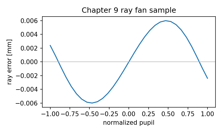
A ray fan does not only show the two-dimensional distribution of errors. It plots error as a function of pupil coordinate.

That is what makes it diagnostic.

Why ray fans reveal structure

A spot diagram answers:

Where did the rays land?

A ray fan asks:

How does the landing error change as we move across the pupil?

That is a more structured question.

For a tangential fan, we may vary one pupil coordinate across a line:

Px from -1 to +1, Py = 0

Then plot image error against Px.

For a sagittal fan, we vary the other pupil coordinate:

Py from -1 to +1, Px = 0

Then plot image error against Py.

A ray fan is therefore built from line samples through the pupil, not necessarily from a full two-dimensional grid.

This is why ray fans can show aberration patterns more clearly than a dense spot diagram. A spot diagram may look like a cloud. A ray fan shows the functional relationship:

pupil coordinate → transverse error

If the error is mostly a straight line, that often indicates defocus. If it curves with a cubic shape, spherical aberration may be present. If the off-axis fan is asymmetric, coma may be involved. If tangential and sagittal fans behave differently, astigmatism or field curvature may be part of the story.

We will not overclaim from one plot. But we can begin to read the shapes.

Sampling a line across the pupil

Let us create line samples across the pupil.

For an x fan:

x varies from -R to +R
y = 0

For a y fan:

x = 0
y varies from -R to +R

In normalized pupil coordinates, we use:

P = coordinate / pupil_radius

so P runs from -1 to +1.

def sample_pupil_line(axis, num_points, pupil_radius):
    """Sample a line through the circular pupil.

    axis:
        "x" for x-line samples with y = 0.
        "y" for y-line samples with x = 0.
    """
    P = np.linspace(-1.0, 1.0, num_points)
    points = []

    for p in P:
        if axis == "x":
            points.append((p * pupil_radius, 0.0))
        elif axis == "y":
            points.append((0.0, p * pupil_radius))
        else:
            raise ValueError("axis must be 'x' or 'y'")

    return P, np.array(points, dtype=float)

We force the number of points to be odd if we want the center ray included:

def odd_count(n):
    return n if n % 2 == 1 else n + 1

Now make a line bundle:

def make_line_bundle(
    axis,
    num_points,
    pupil_radius,
    z_start,
    theta_x_deg=0.0,
    theta_y_deg=0.0,
    wavelength_um=0.5875618,
):
    num_points = odd_count(num_points)
    P, pupil_points = sample_pupil_line(axis, num_points, pupil_radius)

    rays = make_ray_bundle(
        pupil_points=pupil_points,
        z_start=z_start,
        theta_x_deg=theta_x_deg,
        theta_y_deg=theta_y_deg,
        wavelength_um=wavelength_um,
    )

    return P, rays

This gives us both the normalized pupil coordinates and the rays.

Building a ray fan from our singlet tracer

We can now trace a line bundle through the simple singlet from the previous chapters.

Assume we still have:

front
back
image
N_BK7
trace_bundle_through_singlet(...)
collect_image_points(...)

Now write a ray fan function.

def ray_fan_for_singlet(
    axis,
    num_points,
    pupil_radius,
    z_start,
    theta_x_deg,
    theta_y_deg,
    wavelength_um,
    front,
    back,
    image,
    glass_material,
    reference="centroid",
):
    """Compute a simple transverse ray fan for the singlet.

    Returns:
        P: normalized pupil coordinates
        errors: transverse errors, shape (N, 2), for valid rays
        points: image-plane intercepts
        valid_mask: Boolean mask for rays that reached the image plane
        ref: reference point used for transverse error
    """
    P, rays = make_line_bundle(
        axis=axis,
        num_points=num_points,
        pupil_radius=pupil_radius,
        z_start=z_start,
        theta_x_deg=theta_x_deg,
        theta_y_deg=theta_y_deg,
        wavelength_um=wavelength_um,
    )

    traced = trace_bundle_through_singlet(
        rays,
        front=front,
        back=back,
        image=image,
        glass_material=glass_material,
    )

    points = []
    valid_P = []

    for p, ray in zip(P, traced):
        if ray.alive:
            points.append((ray.position[0], ray.position[1]))
            valid_P.append(p)

    points = np.array(points, dtype=float)
    valid_P = np.array(valid_P, dtype=float)

    if len(points) == 0:
        return valid_P, points, points, np.array([], dtype=bool), np.array([np.nan, np.nan])

    if reference == "centroid":
        errors, ref = transverse_errors(points)
    elif reference == "chief":
        # With odd line sampling, the center point is the closest chief-like sample
        center_index = np.argmin(np.abs(valid_P))
        ref = points[center_index]
        errors, ref = transverse_errors(points, reference=ref)
    else:
        raise ValueError("reference must be 'centroid' or 'chief'")

    return valid_P, errors, points, ref

Now plot the fan.

For an on-axis field, use an x fan:

P, errors, points, ref = ray_fan_for_singlet(
    axis="x",
    num_points=51,
    pupil_radius=5.0,
    z_start=-20.0,
    theta_x_deg=0.0,
    theta_y_deg=0.0,
    wavelength_um=0.5875618,
    front=front,
    back=back,
    image=image,
    glass_material=N_BK7,
    reference="chief",
)

plt.plot(P, errors[:, 0], marker=".")
plt.axhline(0.0, linewidth=0.8)
plt.axvline(0.0, linewidth=0.8)
plt.xlabel("normalized pupil coordinate P_x")
plt.ylabel("transverse error εx [mm]")
plt.title("On-axis x ray fan")
plt.show()

That plot is a ray fan.

It is not a new kind of physics. It is a different organization of the same traced ray data.

ray trace → image intercepts → subtract reference → plot error versus pupil coordinate

That is the whole construction.

Defocus: the simplest ray fan shape

Before naming complicated aberrations, start with defocus.

Suppose a bundle would ideally focus at one plane, but we measure it at a plane before or after focus. Then ray intercepts shift roughly linearly with pupil coordinate. Edge rays land on one side, center rays near the reference, opposite edge rays on the other side.

The ray fan becomes approximately a straight line.

This is easy to simulate by moving the image plane.

def make_image_plane(z_image):
    return IntersectableSurface(
        radius=float("inf"),
        z_vertex=z_image,
        semi_diameter=None,
        surface_type="plane",
        comment="image plane",
    )

Now compare fans at different image positions:

for z_image in [40.0, 50.0, 60.0]:
    image_test = make_image_plane(z_image)

    P, errors, points, ref = ray_fan_for_singlet(
        axis="x",
        num_points=51,
        pupil_radius=5.0,
        z_start=-20.0,
        theta_x_deg=0.0,
        theta_y_deg=0.0,
        wavelength_um=0.5875618,
        front=front,
        back=back,
        image=image_test,
        glass_material=N_BK7,
        reference="chief",
    )

    plt.plot(P, errors[:, 0], marker=".", label=f"z={z_image:.0f} mm")

plt.axhline(0.0, linewidth=0.8)
plt.axvline(0.0, linewidth=0.8)
plt.xlabel("normalized pupil coordinate P_x")
plt.ylabel("transverse error εx [mm]")
plt.title("Defocus changes the slope of the ray fan")
plt.legend()
plt.show()

The main change is often a linear tilt in the fan.

This is useful because defocus can mask other patterns. If the image plane is not at a meaningful focus, the ray fan may be dominated by a straight-line term. Once you refocus, the residual curvature becomes easier to inspect.

This is why optical analysis software often lets you change focus or subtract certain reference terms. The plot is not just a raw truth. It is a diagnostic view.

Spherical aberration: edge rays do not focus like near-axis rays

Spherical aberration is one of the most natural aberrations to see with our current code.

For an on-axis object point, a perfect paraxial model would bring all incoming parallel rays to the same focus. A real spherical surface does not generally do that. Rays hitting the lens near the edge may cross the axis at a different z position than rays near the center.

In a ray fan, spherical aberration often appears as a curved pattern, commonly with a cubic-like shape in transverse ray error versus pupil coordinate.

Let us compute approximate axis crossing after the singlet for different input heights.

def trace_simple_singlet_to_exit(ray, front, back, glass_material):
    n_air = 1.0
    n_glass = glass_material.n(ray.wavelength_um)

    interact_refractive_surface(ray, front, n1=n_air, n2=n_glass)

    if ray.alive:
        interact_refractive_surface(ray, back, n1=n_glass, n2=n_air)

    return ray

def z_axis_crossing_xz(ray):
    """Estimate where a ray in the x-z plane crosses x=0 after exit."""
    x0 = ray.position[0]
    z0 = ray.position[2]
    dx = ray.direction[0]
    dz = ray.direction[2]

    if abs(dx) < 1e-12:
        return math.inf

    t = -x0 / dx

    if t < 0:
        return math.inf

    return z0 + t * dz

Now sweep ray height:

heights = np.linspace(0.5, 8.0, 16)
crossings = []

for h in heights:
    ray = Ray(
        position=[h, 0.0, -20.0],
        direction=[0.0, 0.0, 1.0],
        wavelength_um=0.5875618,
    )

    trace_simple_singlet_to_exit(ray, front, back, N_BK7)
    crossings.append(z_axis_crossing_xz(ray))

plt.plot(heights, crossings, marker=".")
plt.xlabel("input ray height [mm]")
plt.ylabel("axis crossing z [mm]")
plt.title("Longitudinal focus shift with ray height")
plt.show()

If the crossing position changes with ray height, the lens has spherical aberration under this setup.

That statement is not a label pulled from memory. It follows from the data:

near-axis rays focus here
edge rays focus somewhere else

This is spherical aberration in computational form.

Transverse spherical aberration at a fixed image plane

Axis crossing is a longitudinal view. A ray fan at a fixed image plane gives a transverse view.

Pick an image plane. Trace rays across the pupil. Plot transverse error.

image_focus = make_image_plane(50.0)

P, errors, points, ref = ray_fan_for_singlet(
    axis="x",
    num_points=101,
    pupil_radius=5.0,
    z_start=-20.0,
    theta_x_deg=0.0,
    theta_y_deg=0.0,
    wavelength_um=0.5875618,
    front=front,
    back=back,
    image=image_focus,
    glass_material=N_BK7,
    reference="chief",
)

plt.plot(P, errors[:, 0])
plt.axhline(0.0, linewidth=0.8)
plt.axvline(0.0, linewidth=0.8)
plt.xlabel("normalized pupil coordinate P_x")
plt.ylabel("transverse error εx [mm]")
plt.title("On-axis transverse ray fan")
plt.show()

For a rotationally symmetric on-axis system, the x fan and y fan should behave similarly. If the plot is curved and symmetric in the expected way, you are seeing how ray height changes focus and image-plane intercept.

Do not worry about naming every coefficient. The computational interpretation is enough:

the error is not constant
the error is not only a linear defocus term
the error varies with pupil coordinate

That variation is the ray trace exposing aberration.

Coma: off-axis asymmetry

Now move off-axis.

Coma appears for off-axis field points when rays from different pupil zones produce an asymmetric blur. In a spot diagram, coma can look like a comet: a dense head and a spreading tail. In ray fan plots, coma introduces asymmetric terms that are not present for the on-axis symmetric case.

Let us trace an off-axis field:

image_focus = make_image_plane(50.0)

P, errors, points, ref = ray_fan_for_singlet(
    axis="y",
    num_points=101,
    pupil_radius=5.0,
    z_start=-20.0,
    theta_x_deg=0.0,
    theta_y_deg=5.0,
    wavelength_um=0.5875618,
    front=front,
    back=back,
    image=image_focus,
    glass_material=N_BK7,
    reference="chief",
)

plt.plot(P, errors[:, 1])
plt.axhline(0.0, linewidth=0.8)
plt.axvline(0.0, linewidth=0.8)
plt.xlabel("normalized pupil coordinate P_y")
plt.ylabel("transverse error εy [mm]")
plt.title("Off-axis ray fan")
plt.show()

Now also plot the off-axis spot:

pupil_points = sample_pupil_grid(samples_per_axis=17, pupil_radius=5.0)

rays = make_ray_bundle(
    pupil_points=pupil_points,
    z_start=-20.0,
    theta_x_deg=0.0,
    theta_y_deg=5.0,
    wavelength_um=0.5875618,
)

traced = trace_bundle_through_singlet(rays, front, back, image_focus, N_BK7)
spot_points, valid = collect_image_points(traced)
spot_errors, ref = transverse_errors(spot_points)

plot_spot(spot_errors, title="Off-axis spot, centered")

If the centered spot is asymmetric, that is a clue. If the ray fan shows asymmetric departure as pupil coordinate changes, that is another clue.

This is the practical way to meet coma:

not as a word first,
but as an off-axis asymmetric error pattern in traced ray data.

A simple singlet is not corrected for off-axis aberrations, so it is a good teaching object. It behaves badly enough to show the problem.

Tangential and sagittal behavior

Off-axis systems have a special complication.

There are two important planes:

tangential plane
sagittal plane

If the field is in the y direction, the tangential plane contains the optical axis and the field direction. The sagittal plane is perpendicular to it.

In practical ray fan terms, we often inspect two fans:

tangential fan
sagittal fan

The exact naming depends on coordinate convention. The important computational idea is:

Sample rays along two orthogonal pupil lines and compare their transverse errors.

If the tangential and sagittal fans behave differently, the system is telling you that off-axis imaging is not the same in the two planes.

That difference is connected to astigmatism and field curvature.

Let us compute both line fans for the same off-axis field:

field_angle = 5.0
image_focus = make_image_plane(50.0)

P_x, errors_x, points_x, ref_x = ray_fan_for_singlet(
    axis="x",
    num_points=101,
    pupil_radius=5.0,
    z_start=-20.0,
    theta_x_deg=0.0,
    theta_y_deg=field_angle,
    wavelength_um=0.5875618,
    front=front,
    back=back,
    image=image_focus,
    glass_material=N_BK7,
    reference="chief",
)

P_y, errors_y, points_y, ref_y = ray_fan_for_singlet(
    axis="y",
    num_points=101,
    pupil_radius=5.0,
    z_start=-20.0,
    theta_x_deg=0.0,
    theta_y_deg=field_angle,
    wavelength_um=0.5875618,
    front=front,
    back=back,
    image=image_focus,
    glass_material=N_BK7,
    reference="chief",
)

plt.plot(P_x, errors_x[:, 0], label="x fan: εx")
plt.plot(P_y, errors_y[:, 1], label="y fan: εy")
plt.axhline(0.0, linewidth=0.8)
plt.axvline(0.0, linewidth=0.8)
plt.xlabel("normalized pupil coordinate")
plt.ylabel("transverse error [mm]")
plt.title("Two orthogonal ray fans for an off-axis field")
plt.legend()
plt.show()

This comparison is more informative than either curve alone.

If one plane focuses differently from the other, moving the image plane may improve one fan while worsening the other. That is the practical sign of astigmatic behavior.

Astigmatism: two line foci instead of one point focus

Astigmatism does not mean “everything is blurry” in a generic way.

For an off-axis field, rays in two orthogonal sections of the bundle may come to best focus at different axial positions. Instead of one clean point focus, the system has two preferred line-like foci: tangential and sagittal.

A simple way to see this computationally is to scan image plane position and compute RMS width in two directions.

Let us use off-axis ray bundles and measure spot spread as the image plane moves.

def spot_statistics_for_plane(z_image, field_angle, wavelength_um=0.5875618):
    image_test = make_image_plane(z_image)
    pupil_points = sample_pupil_grid(samples_per_axis=17, pupil_radius=5.0)

    rays = make_ray_bundle(
        pupil_points=pupil_points,
        z_start=-20.0,
        theta_x_deg=0.0,
        theta_y_deg=field_angle,
        wavelength_um=wavelength_um,
    )

    traced = trace_bundle_through_singlet(rays, front, back, image_test, N_BK7)
    points, valid = collect_image_points(traced)

    if len(points) == 0:
        return np.nan, np.nan, np.nan

    centered, ref = transverse_errors(points)
    rms_x = math.sqrt(float(np.mean(centered[:, 0]**2)))
    rms_y = math.sqrt(float(np.mean(centered[:, 1]**2)))
    rms_r = rms_spot_radius(points)

    return rms_x, rms_y, rms_r

Sweep focus:

z_values = np.linspace(35.0, 70.0, 71)
field_angle = 5.0

rms_x_values = []
rms_y_values = []
rms_r_values = []

for z in z_values:
    rms_x, rms_y, rms_r = spot_statistics_for_plane(z, field_angle)
    rms_x_values.append(rms_x)
    rms_y_values.append(rms_y)
    rms_r_values.append(rms_r)

plt.plot(z_values, rms_x_values, label="RMS x")
plt.plot(z_values, rms_y_values, label="RMS y")
plt.plot(z_values, rms_r_values, label="RMS radius")
plt.xlabel("image plane z [mm]")
plt.ylabel("RMS spot size [mm]")
plt.title("Focus scan for an off-axis field")
plt.legend()
plt.show()

If the minima of RMS x and RMS y occur at different z positions, the system has different best focus behavior in two transverse directions.

That is the computational flavor of astigmatism.

Again, we are not asking you to memorize a diagram. We are showing how a ray trace reveals the effect.

Field curvature: best focus changes across the field

A flat sensor is flat. Real optical systems may prefer a curved image surface.

Field curvature means that the best focus position changes with field. The center field might focus at one image plane, while the edge field wants another.

This is easy to confuse with ordinary defocus unless you compare multiple field points.

Let us compute the best RMS focus for several fields.

def best_focus_by_rms(field_angle, z_min=35.0, z_max=70.0, count=71):
    z_values = np.linspace(z_min, z_max, count)
    rms_values = []

    for z in z_values:
        _, _, rms_r = spot_statistics_for_plane(z, field_angle)
        rms_values.append(rms_r)

    rms_values = np.array(rms_values)
    idx = np.nanargmin(rms_values)

    return z_values[idx], rms_values[idx], z_values, rms_values

Run it:

for field_angle in [0.0, 2.0, 4.0, 6.0]:
    z_best, rms_best, _, _ = best_focus_by_rms(field_angle)
    print(
        f"field={field_angle:.1f} deg, "
        f"best z≈{z_best:.2f} mm, "
        f"best RMS≈{rms_best:.6f} mm"
    )

If best focus shifts with field, that is field curvature in computational terms.

A flat image plane cannot satisfy every field perfectly if the best-focus surface is curved. A designer may accept this, correct it, or balance it against other aberrations. A camera lens, microscope objective, eyepiece, or projection lens may care about this differently.

The key point is simple:

field curvature is not just blur at the edge.
It is a field-dependent best-focus position.

A focus scan makes that visible.

Distortion: image position is wrong even if the spot is sharp

Distortion is different from blur.

A lens can form a relatively sharp image point at the wrong location. That is distortion.

This is why a centered spot diagram can hide distortion. If you subtract the centroid or chief ray intercept, you remove the image displacement and look only at spread. That is useful for blur, but not for mapping accuracy.

To see distortion, compare real image height with paraxial image height.

From Chapter 8:

y_paraxial ≈ f tan θ

For our simple singlet, we can use a thin-lens focal length estimate as a rough reference. A real library’s paraxial analysis would give a better reference from the actual prescription, but the thin-lens estimate is enough to show the method.

def real_chief_ray_image_height(field_angle_deg, z_image, wavelength_um=0.5875618):
    image_test = make_image_plane(z_image)

    chief = make_chief_ray(
        z_start=-20.0,
        theta_x_deg=0.0,
        theta_y_deg=field_angle_deg,
        wavelength_um=wavelength_um,
    )

    trace_simple_singlet_ray(chief, front, back, image_test, N_BK7)

    if not chief.alive:
        return np.nan

    return chief.position[1]

Now compare:

f_est = thin_lens_focal_length_from_radii(
    N_BK7.n(0.5875618),
    R1=50.0,
    R2=-50.0,
)

z_image = 50.0

for field_angle in [1.0, 2.0, 3.0, 5.0, 7.0]:
    y_real = real_chief_ray_image_height(field_angle, z_image)
    y_para = paraxial_image_height_from_field(f_est, field_angle)
    error = y_real - y_para

    print(
        f"field={field_angle:.1f} deg, "
        f"real y={y_real:.4f} mm, "
        f"paraxial y={y_para:.4f} mm, "
        f"distortion-like error={error:.4f} mm"
    )

This is not a polished distortion analysis. The focal length reference is crude, and our simple chief ray model is simplified. But the structure is correct:

field angle
→ paraxial image height
→ real chief ray image height
→ difference

That difference is mapping error.

The spot could be tiny and the mapping could still be distorted. That is why distortion belongs in the aberration family but behaves differently from blur.

Chromatic aberration: different wavelengths, different rays

Chromatic aberration comes from the material model.

In Chapter 3, we learned that glass refractive index depends on wavelength:

n = n(λ)

In Chapter 6, we used that index in Snell’s law.

Therefore rays of different wavelengths do not trace exactly the same path through the same lens.

There are two common chromatic effects to notice:

longitudinal chromatic aberration:
    different wavelengths focus at different axial positions

lateral chromatic aberration:
    different wavelengths have different image heights off-axis

Let us compute a simple longitudinal chromatic focus estimate.

for wl in [0.4861327, 0.5875618, 0.6562725]:
    z_best, rms_best, _, _ = best_focus_by_rms(
        field_angle=0.0,
        z_min=35.0,
        z_max=70.0,
        count=71,
    )
    print(wl, z_best, rms_best)

This version accidentally uses the default wavelength inside spot_statistics_for_plane, so let us make the wavelength explicit.

def best_focus_by_rms_for_wavelength(
    field_angle,
    wavelength_um,
    z_min=35.0,
    z_max=70.0,
    count=71,
):
    z_values = np.linspace(z_min, z_max, count)
    rms_values = []

    for z in z_values:
        rms_x, rms_y, rms_r = spot_statistics_for_plane(
            z_image=z,
            field_angle=field_angle,
            wavelength_um=wavelength_um,
        )
        rms_values.append(rms_r)

    rms_values = np.array(rms_values)
    idx = np.nanargmin(rms_values)

    return z_values[idx], rms_values[idx]

Now compute:

for wl in [0.4861327, 0.5875618, 0.6562725]:
    z_best, rms_best = best_focus_by_rms_for_wavelength(
        field_angle=0.0,
        wavelength_um=wl,
    )

    print(
        f"λ={wl:.7f} µm, "
        f"best focus z≈{z_best:.2f} mm, "
        f"best RMS≈{rms_best:.6f} mm"
    )

If the best focus differs by wavelength, you are seeing longitudinal chromatic aberration.

For lateral chromatic aberration, compare off-axis chief ray image heights by wavelength:

field_angle = 5.0
z_image = 50.0

for wl in [0.4861327, 0.5875618, 0.6562725]:
    y_real = real_chief_ray_image_height(
        field_angle_deg=field_angle,
        z_image=z_image,
        wavelength_um=wl,
    )

    print(f"λ={wl:.7f} µm, chief ray image y={y_real:.6f} mm")

If image height changes with wavelength, that is lateral color in this simplified analysis.

The singlet is not meant to look good. It will not. It is useful because chromatic aberration emerges from the same ray-tracing machinery.

No special “chromatic aberration module” is needed at the conceptual level.

The chain is:

wavelength
→ refractive index
→ refracted direction
→ image intercept
→ wavelength-dependent focus or image height

A taxonomy from computations, not from memorization

Now we can summarize the classical aberrations in computational terms.

Spherical aberration

On-axis rays at different pupil radii focus differently.

Computational sign:

axis crossing z changes with pupil height
on-axis ray fan shows curved error versus pupil coordinate

Coma

Off-axis rays form an asymmetric blur.

Computational sign:

off-axis spot becomes asymmetric
off-axis ray fan shows asymmetric error terms

Astigmatism

Tangential and sagittal sections focus differently.

Computational sign:

two orthogonal fan directions behave differently
RMS x and RMS y may have minima at different image planes

Field curvature

Best focus changes with field.

Computational sign:

best RMS focus z shifts as field angle changes
flat image plane cannot match all fields equally

Distortion

Image point is displaced from the paraxial mapping, even if the spot is sharp.

Computational sign:

real chief ray or centroid image height differs from paraxial image height
centered spot diagram may hide it

Chromatic aberration

Different wavelengths image differently.

Computational sign:

best focus shifts with wavelength
off-axis image height changes with wavelength
polychromatic spot separates by color

This way of learning aberrations is slower than memorizing a table. It is also sturdier.

The names now attach to measured behavior.

Why real ray fans are not wavefront maps

A ray fan plot is powerful, but it is still ray-based.

It plots transverse image error versus pupil coordinate. It does not directly show optical path difference. It does not by itself give PSF or MTF. It is still part of geometric optics.

That limitation matters.

Two systems with similar spot diagrams may have different wavefront phase behavior. Diffraction can dominate when geometric spots become small. A lens near diffraction-limited performance needs wavefront analysis, not only ray intercepts.

So this chapter is a bridge, but not the final bridge.

We have moved from:

where do rays land?

to:

how do real rays depart from a reference?

The next chapter moves to:

how do ray paths become optical path difference across the pupil?

That is the bridge from geometric ray tracing to wave optics.

Optiland RayFan as a higher-level version

A real optical library already has ray fan tools.

In current Optiland documentation, the RayFan analysis takes an optic, fields, wavelengths, and a number of points; it traces line distributions across the pupil and stores x and y ray fan data. The source also shows that the standard view plots ray fan error against normalized pupil coordinates, with separate x and y fan panels. (Optiland)

A compact Optiland-style workflow looks like this:

from optiland.samples.objectives import CookeTriplet
from optiland.analysis import RayFan

lens = CookeTriplet()

fan = RayFan(
    lens,
    fields="all",
    wavelengths="all",
    num_points=101,
)

fan.view()

For a custom singlet, the setup would follow the same optical-system construction style used earlier:

from optiland import optic
from optiland.analysis import RayFan

lens = optic.Optic()

lens.surfaces.add(index=0, radius=float("inf"), thickness=float("inf"))
lens.surfaces.add(index=1, radius=50.0, thickness=5.0, material="N-BK7", is_stop=True)
lens.surfaces.add(index=2, radius=-50.0, thickness=45.0)
lens.surfaces.add(index=3)

lens.set_aperture(aperture_type="EPD", value=10.0)
lens.fields.set_type("angle")
lens.fields.add(y=0.0)
lens.fields.add(y=5.0)
lens.wavelengths.add(value=0.5876, is_primary=True)

fan = RayFan(lens, fields="all", wavelengths="all", num_points=101)
fan.view()

Treat this as library-level comparison code. Exact import paths and options can change as the project evolves, but the computational meaning is stable:

select field and wavelength
trace line samples through the pupil
measure image-plane transverse error
plot error versus normalized pupil coordinate

The current Optiland source also includes a BestFitRayFan class that references ray fan data to a best-fit sphere center rather than the ordinary chief-ray-centered reference. That is a useful reminder that ray fan plots depend on reference convention, not only on traced rays. (Optiland)

This is exactly why we built the small version ourselves first.

When a library gives you a beautiful fan plot, you can now ask:

What pupil line was sampled?
What field and wavelength were used?
What reference point was subtracted?
Was distortion removed?
Were invalid rays suppressed?

Those questions are not pedantic. They determine what the plot means.

A small diagnostic workflow

When reading ray fan results, use a disciplined order.

First, check the setup:

field
wavelength
aperture
image plane
reference convention
sampling density

Second, check whether rays were lost:

blocked by aperture
missed a surface
total internal reflection
invalid image intercept

Third, separate defocus from residual shape. If the fan is mostly a straight line, move the image plane or subtract focus before diagnosing more subtle aberrations.

Fourth, compare x and y fans. Do not assume one fan tells the full story.

Fifth, compare fields. On-axis and off-axis behavior are often completely different.

Sixth, compare wavelengths. If the curves separate by wavelength, the material model is speaking.

Finally, connect the fan to the spot diagram. The fan explains structure. The spot shows the two-dimensional landing pattern. Neither replaces the other.

This workflow is more reliable than trying to recognize every aberration by visual memory alone.

Common mistakes when interpreting aberrations

Let us name the traps clearly.

Mistake 1: Calling every blur “spherical aberration”

Spherical aberration is specifically about how ray behavior changes with pupil radius for an on-axis field. Off-axis blur may involve coma, astigmatism, field curvature, and other effects.

Mistake 2: Forgetting the image plane

A ray fan can be dominated by defocus if the image plane is poorly chosen. Before diagnosing subtle aberrations, check focus.

Mistake 3: Centering away distortion

A centered spot or chief-ray-referenced fan may remove image displacement. That is useful for blur analysis, but it can hide distortion.

Mistake 4: Comparing fans with different references

A fan referenced to the chief ray is not the same as a fan referenced to a paraxial image point or best-fit focus.

Mistake 5: Ignoring wavelength

A monochromatic fan cannot show chromatic separation. A polychromatic fan may contain several overlapping stories.

Mistake 6: Reading a sparse fan too confidently

Sampling density matters. Too few points can hide curvature or make a curve look cleaner than it is.

Mistake 7: Treating ray fans as diffraction analysis

Ray fans are geometric. They do not directly tell you the diffraction PSF or MTF.

Mistake 8: Forgetting units

A fan error of 0.01 mm may be large or small depending on pixel size, Airy disk size, focal length, and intended use.

Mistake 9: Expecting a simple singlet to behave like a corrected objective

A biconvex singlet is a teaching system. It will show aberrations clearly because it is not corrected. That is useful here.

Mistake 10: Diagnosing from one plot alone

Use spot diagrams, ray fans, focus scans, field comparisons, and wavelength comparisons together. One plot rarely tells the whole truth.

What this chapter gives us

We now have a computational way to discuss aberration.

We can:

trace real rays through a lens
choose a reference intercept
compute transverse ray error
sample line fans across the pupil
plot ray fan curves
scan focus position
compare fields
compare wavelengths
connect ray fan shapes to classical aberrations

The important shift is this:

Aberrations are no longer just names. They are patterns in computed ray error.

This is the right level of understanding for the rest of the book.

When we later compute OPD, PSF, OTF, and MTF, we will not forget the ray story. Wave optics does not erase geometric optics. It extends it. The wavefront across the pupil is built from optical path differences, and those paths come from traced rays through the system.

Ray fans tell us how rays miss.

Wavefront maps will tell us how phase departs.

PSF will show how a point spreads.

MTF will show how contrast survives.

The chain is getting longer, but each link is now visible.

The road ahead

The ray fan is a powerful diagnostic, but it still lives in image-plane coordinates. It tells us transverse error.

To reach diffraction analysis, we need a different quantity.

We need optical path difference.

A ray does not only land somewhere. It also accumulates optical path length as it travels through air and glass. Different rays across the pupil may arrive with different optical path lengths relative to a reference wavefront. That difference becomes phase error.

That is the bridge from ray tracing to wave optics.

The next chapter will therefore ask:

How do we turn traced ray paths into OPD across the pupil?

Once we have OPD, the later chapters can build the pupil function, PSF, OTF, and finally MTF.

A spot diagram comes from where rays land.

A wavefront map comes from how much optical path they carry.

We now know the first. Next, we learn the second.

Generated validation figure