Chapter 8: Why Paraxial Optics Still Matters
We have just built real ray tracing.
That feels like progress, and it is. A ray can now start from a pupil coordinate, travel to a spherical surface, find the local normal, refract through glass, leave the lens, and land on an image plane. A bundle of such rays can produce a spot diagram.
So it may feel odd to step backward now.
Why talk about paraxial optics after real rays?
Why return to thin lenses, small angles, focal length, F-number, numerical aperture, and ABCD matrices when we already have a more exact ray tracer?
Because paraxial optics is not a primitive substitute for real ray tracing.
It is the skeleton.
Real ray tracing tells us what the rays actually do. Paraxial optics tells us what the system is trying to do in first-order form. Without that skeleton, spot diagrams can become isolated pictures. You may see that rays spread, but not know what they are spreading around. You may see that focus changes, but not know which first-order focus the real rays are departing from.
A spot diagram says:
Here is where sampled real rays landed.
Paraxial optics says:
Here is the ideal first-order image structure the system is organized around.
Both are needed.
This chapter introduces the paraxial reference system: ray height, ray slope, transfer matrices, thin lenses, effective focal length, back focal length, F-number, numerical aperture, and magnification. The model stays deliberately small. It gives us the reference frame needed for the next chapter, not a replacement for an optical design textbook.
Chapter 9 will ask:
Why do real rays depart from paraxial rays?
That question is the beginning of aberration.
So first we need to understand the paraxial ray.
A paraxial ray is a reduced description
A real ray in our code carries a 3D position and a 3D direction:
position  = [x, y, z]
direction = [dx, dy, dz]
A paraxial ray is simpler.
In one transverse plane, it can be represented by:
y = ray height
u = ray angle or slope
Here y is the height above the optical axis, and u is the small angle the ray makes with the optical axis.
For small angles:
sin u ≈ u
tan u ≈ u
when u is measured in radians.
That small-angle approximation is the heart of paraxial optics.
This approximation does not mean paraxial optics is careless. It means paraxial optics intentionally studies rays close to the optical axis and close to small angles. That is enough to reveal the first-order behavior of the system.
A real ray answers:
Where does this actual ray go through the actual surface?
A paraxial ray answers:
How does a near-axis ray behave under the first-order approximation?
Those are different questions.
Both are useful.
The paraxial ray vector
We will write a paraxial ray as a two-element vector:
[y, u]
where:
y = height above the optical axis, in mm
u = slope or small angle, in radians
In code:
from dataclasses import dataclass
import numpy as np
import math

@dataclass
class ParaxialRay:
    y: float
    u: float  # radians, or slope under small-angle approximation

    def as_vector(self):
        return np.array([self.y, self.u], dtype=float)

    @classmethod
    def from_vector(cls, v):
        return cls(y=float(v[0]), u=float(v[1]))
A ray traveling parallel to the optical axis at height 5 mm is:
ray = ParaxialRay(y=5.0, u=0.0)
A ray crossing the axis with a small downward angle might be:
ray = ParaxialRay(y=5.0, u=-0.05)
This is much less information than a real ray. That is the point. The paraxial ray is a simplified carrier of first-order behavior.
Propagation in paraxial form
If a paraxial ray travels a distance d through a uniform medium, its height changes according to its slope:
y_new = y + d u
Its slope remains the same:
u_new = u
That can be written as a matrix:
[ y_new ]   [ 1  d ] [ y ]
[ u_new ] = [ 0  1 ] [ u ]
This is the first ABCD matrix.
The propagation matrix is:
T(d) = [[1, d],
        [0, 1]]
In code:
def translation_matrix(distance):
    """Paraxial propagation through distance d in a uniform medium."""
    return np.array([
        [1.0, distance],
        [0.0, 1.0],
    ], dtype=float)

def apply_matrix(M, ray):
    """Apply a 2x2 paraxial matrix to a ParaxialRay."""
    return ParaxialRay.from_vector(M @ ray.as_vector())
Test it:
ray = ParaxialRay(y=5.0, u=-0.1)

M = translation_matrix(20.0)
out = apply_matrix(M, ray)

print(out)
The result should be:
y = 3.0
u = -0.1
because:
5 + 20 × (-0.1) = 3
This is not a rough drawing. It is the first-order ray transfer written as code.
A thin lens matrix
A thin lens changes the slope of a ray but not its height at the lens plane.
For a thin lens with focal length f in air:
y_new = y
u_new = u - y / f
The matrix is:
L(f) = [[1,    0],
        [-1/f, 1]]
In code:
def thin_lens_matrix(focal_length):
    """Thin lens matrix in air."""
    f = float(focal_length)

    if f == 0:
        raise ValueError("Focal length cannot be zero.")

    return np.array([
        [1.0, 0.0],
        [-1.0 / f, 1.0],
    ], dtype=float)
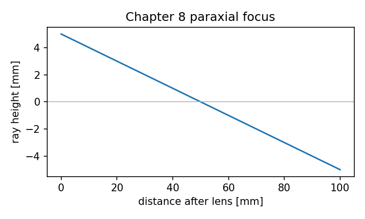
Test a parallel ray hitting a 50 mm thin lens at height 5 mm:
ray = ParaxialRay(y=5.0, u=0.0)

L = thin_lens_matrix(50.0)
out = apply_matrix(L, ray)

print(out)
The outgoing slope is:
u_new = -5 / 50 = -0.1
That means the ray now travels downward toward the axis. If it propagates 50 mm, it reaches the axis:
T = translation_matrix(50.0)

after_focus = apply_matrix(T, out)
print(after_focus)
The height should be near zero.
This is the paraxial version of focusing.
It is not using real surface intersections. It is not using the exact spherical surface normals. It is using the first-order model of a lens.
That is why it is so compact.
Matrix multiplication is the optical system
An optical system can be represented as a product of paraxial matrices.
If a ray passes through:
translation d1
thin lens f
translation d2
then:
ray_out = T(d2) L(f) T(d1) ray_in
The rightmost matrix acts first.
So the system matrix is:
M = T(d2) @ L(f) @ T(d1)
In code:
def system_matrix(*matrices):
    """Combine matrices in the order they act on the ray.

    system_matrix(A, B, C) returns C @ B @ A if the ray sees A first,
    then B, then C.
    """
    M = np.eye(2)

    for element in matrices:
        M = element @ M

    return M
This version lets us write elements in physical order:
M = system_matrix(
    translation_matrix(10.0),
    thin_lens_matrix(50.0),
    translation_matrix(40.0),
)
The ray sees 10 mm of propagation, then the lens, then 40 mm more propagation.
This order convention is worth being explicit about. Matrix optics is compact, but order matters. Swapping two elements changes the system.
The ABCD matrix
A general first-order system matrix is written:
M = [[A, B],
     [C, D]]
It maps input ray height and slope to output ray height and slope:
[ y_out ]   [ A  B ] [ y_in ]
[ u_out ] = [ C  D ] [ u_in ]
So:
y_out = A y_in + B u_in
u_out = C y_in + D u_in
Each coefficient has a meaning.
A tells how input height contributes to output height.
B tells how input angle contributes to output height.
C tells how input height contributes to output angle.
D tells how input angle contributes to output angle.
The most important coefficient for optical power is often C.
For a thin lens:
M = [[1,    0],
     [-1/f, 1]]
so:
C = -1/f
That is why, for a system in air, the effective focal length is often obtained from:
EFL = -1 / C
when C is not zero.
Let us write that.
def matrix_elements(M):
    A, B = M[0, 0], M[0, 1]
    C, D = M[1, 0], M[1, 1]
    return A, B, C, D

def effective_focal_length(M):
    """Effective focal length for a system in air using [y, u] convention."""
    A, B, C, D = matrix_elements(M)

    if abs(C) < 1e-12:
        return math.inf

    return -1.0 / C
Test it:
L = thin_lens_matrix(50.0)
print(effective_focal_length(L))
It should print 50.0.
That is reassuring. A 50 mm thin lens has 50 mm effective focal length in this simplified model.
Back focal length
Effective focal length and back focal length are related but not always identical.
Effective focal length is tied to the system’s optical power and principal planes. Back focal length is the distance from the last surface or last reference plane to the rear focal point.
For a system matrix M = [[A, B], [C, D]], consider an incoming collimated ray:
u_in = 0
After the system:
y_out = A y_in
u_out = C y_in
Now let the ray propagate a distance s after the system. Its height becomes:
y(s) = y_out + s u_out
The rear focal point is where this collimated input ray crosses the axis:
0 = A y_in + s C y_in
For nonzero y_in:
s = -A / C
So, in this simple same-medium convention:
BFL = -A / C
Write it:
def back_focal_length(M):
    """Back focal length from the output reference plane, in air."""
    A, B, C, D = matrix_elements(M)

    if abs(C) < 1e-12:
        return math.inf

    return -A / C
For a thin lens whose reference plane is at the lens itself:
L = thin_lens_matrix(50.0)

print("EFL:", effective_focal_length(L))
print("BFL:", back_focal_length(L))
Both are 50 mm.
Now add a translation after the lens into the system matrix:
M = system_matrix(
    thin_lens_matrix(50.0),
    translation_matrix(10.0),
)

print(M)
print("EFL:", effective_focal_length(M))
print("BFL from output plane:", back_focal_length(M))
The effective focal length remains 50 mm, because the optical power did not change. But the back focal length measured from the new output plane changes. If the output plane is 10 mm after the thin lens, the remaining distance to focus is about 40 mm.
This is a crucial distinction.
A system can have the same effective focal length but a different back focal length depending on where the last reference plane or last surface is.
That is why optical prescriptions care about surface positions, not just power.
Thin lens formula from matrices
The familiar thin lens formula is:
1/s + 1/s' = 1/f
where:
s  = object distance before the lens
s' = image distance after the lens
f  = focal length
Sign conventions vary, so this formula is often a source of confusion. Instead of arguing with signs abstractly, let us derive a simple case using matrices.
Suppose an object point is a distance s before a thin lens. A ray leaves the object point at height 0 and reaches the lens at height y. Its slope at the lens is approximately:
u = y / s
After the thin lens:
u_after = u - y/f
        = y/s - y/f
For the ray to reach the image point on the axis after distance s':
0 = y + s' u_after
Substitute:
0 = y + s'(y/s - y/f)
Divide by y:
0 = 1 + s'(1/s - 1/f)
Rearrange:
1/s' = 1/f - 1/s
or:
1/s + 1/s' = 1/f
under this positive-distance setup.
In code:
def thin_lens_image_distance(object_distance, focal_length):
    """Return image distance s' for a thin lens with object distance s.

    Uses 1/s + 1/s' = 1/f.
    Assumes a simple real-object, real-image positive distance convention.
    """
    s = float(object_distance)
    f = float(focal_length)

    denom = 1.0 / f - 1.0 / s

    if abs(denom) < 1e-12:
        return math.inf

    return 1.0 / denom
Test:
for s in [100.0, 200.0, 1000.0, math.inf]:
    if math.isinf(s):
        sp = 50.0
    else:
        sp = thin_lens_image_distance(s, 50.0)

    print("object distance:", s, "image distance:", sp)
As the object moves farther away, the image distance approaches the focal length.
This is one of the reasons object-at-infinity examples are so convenient. Parallel incoming rays focus at the focal plane in the paraxial thin-lens model.
Magnification
For a thin lens with object distance s and image distance s', transverse magnification is:
m = -s' / s
The minus sign indicates image inversion under the usual real-object, real-image convention.
In code:
def thin_lens_magnification(object_distance, image_distance):
    return -image_distance / object_distance
Example:
s = 100.0
f = 50.0
sp = thin_lens_image_distance(s, f)
m = thin_lens_magnification(s, sp)

print("s' =", sp)
print("m =", m)
For s = 100 mm and f = 50 mm, the image distance is 100 mm and magnification is -1.
Again, this is a first-order result. Real lenses may have distortion, field curvature, aberrations, and finite thickness effects. But the paraxial magnification gives the reference structure.
Without it, “distortion” has no clear meaning. Distortion is not merely “the image looks weird.” It is a departure from the expected paraxial mapping between object field and image position.
We will return to this in Chapter 9.
F-number
F-number is one of the most common optical quantities.
For a lens focused at infinity, a useful first-order definition is:
F/# = f / D
where:
f = effective focal length
D = entrance pupil diameter
A 50 mm lens with a 10 mm entrance pupil diameter has:
F/# = 50 / 10 = 5
or f/5.
In code:
def f_number(effective_focal_length, entrance_pupil_diameter):
    D = float(entrance_pupil_diameter)

    if D <= 0:
        raise ValueError("Entrance pupil diameter must be positive.")

    return effective_focal_length / D
Use it:
f = 50.0
D = 10.0

print(f_number(f, D))
This is simple, but it connects directly to ray bundles.
The entrance pupil diameter controls the cone of rays. A larger aperture means a faster system, smaller F-number, and generally stronger demands on aberration correction. A smaller aperture means a slower system, larger F-number, and often reduced geometric aberrations, but more diffraction blur.
This is one of the places where geometric and diffraction thinking meet.
A large aperture may improve light collection and diffraction-limited resolution, but it also asks the lens to handle more extreme rays. If the design is not corrected, real-ray aberrations may dominate.
F-number is therefore not just a label on a camera lens. It is a first-order summary of aperture relative to focal length.
Numerical aperture
Numerical aperture, or NA, describes the cone angle of light.
In image space, for a medium of refractive index n:
NA = n sin θ
where θ is the marginal ray angle relative to the optical axis.
For small angles in air:
NA ≈ sin θ ≈ θ
There is also a common approximate relationship for systems in air:
NA ≈ 1 / (2 F/#)
when the system is focused at infinity and the angles are not too large.
Let us implement both.
def numerical_aperture(n_medium, marginal_angle_rad):
    return n_medium * math.sin(marginal_angle_rad)

def na_from_f_number(fno):
    return 1.0 / (2.0 * fno)
For a 50 mm focal length and 10 mm entrance pupil diameter:
fno = f_number(50.0, 10.0)

print("F/#:", fno)
print("approx NA:", na_from_f_number(fno))
The approximate NA is 0.1.
This corresponds to a marginal ray angle of about 0.1 radian in the paraxial approximation.
Again, this is first-order. At high NA, exact definitions and sine behavior matter more. But for many introductory optical systems, this approximation gives a useful scale.
F-number connects to the marginal ray
Let us connect F-number to a paraxial ray.
For an object at infinity, a marginal ray enters parallel to the optical axis at pupil height:
y = D / 2
After a thin lens of focal length f, its slope becomes:
u = -y / f = -(D/2) / f
So the marginal ray angle magnitude is approximately:
|u| = D / (2f) = 1 / (2 F/#)
That is the same approximate NA in air.
This is a nice moment because it links several quantities:
pupil diameter
focal length
F-number
marginal ray slope
numerical aperture
They are not separate facts to memorize. They are different views of the first-order cone of light.
In code:
def marginal_slope_from_f_and_d(f, D):
    return -(D / 2.0) / f

f = 50.0
D = 10.0

u_marginal = marginal_slope_from_f_and_d(f, D)

print("marginal slope:", u_marginal)
print("approx NA:", abs(u_marginal))
print("from F/#:", na_from_f_number(f_number(f, D)))
The numbers agree under the paraxial approximation.
This is exactly why paraxial optics is useful. It compresses the geometry into relationships you can reason with.
Real ray marginal behavior versus paraxial marginal behavior
Now connect this chapter to the previous one.
In the real ray tracer, a marginal ray at the edge of the pupil hits the spherical surface at a different normal than a near-axis ray. It refracts according to exact geometry.
In paraxial optics, the marginal ray is represented by a height and a small slope. The lens changes its slope linearly:
u_new = u - y/f
If the ray is near the axis and the angle is small, the two descriptions should be close.
If the ray is far from the axis or the lens has significant aberration, the real ray departs from the paraxial prediction.
That departure is not an inconvenience. It is the beginning of aberration analysis.
A real ray trace gives:
actual image-plane intercept
A paraxial model gives:
first-order expected intercept
The difference gives:
transverse ray error
Chapter 9 will build directly on that idea.
A paraxial focus scan
Let us make a small paraxial focus calculation using matrices.
A collimated ray entering a thin lens at height y should cross the axis at the focal distance. We can verify this by propagating to different z positions and measuring height.
def trace_paraxial_thin_lens_to_plane(y_in, u_in, f, z_after_lens):
    ray = ParaxialRay(y=y_in, u=u_in)

    ray_after_lens = apply_matrix(thin_lens_matrix(f), ray)
    ray_at_plane = apply_matrix(translation_matrix(z_after_lens), ray_after_lens)

    return ray_at_plane
Sweep image plane position:
f = 50.0
y_in = 5.0
u_in = 0.0

z_values = np.linspace(30.0, 70.0, 9)

for z in z_values:
    out = trace_paraxial_thin_lens_to_plane(y_in, u_in, f, z)
    print(f"z={z:.1f} mm, y={out.y:.4f} mm")
At z = 50 mm, the height should be close to zero.
This is the paraxial version of a focus scan. It uses one marginal ray rather than a full bundle. For a thin lens, the result is exact within the paraxial model.
In a real spherical singlet, the edge ray may not cross at exactly the same point as the near-axis ray. That difference is spherical aberration.
Again, paraxial optics gives the reference.
A simple thick-lens approximation with matrices
A real singlet has two surfaces and thickness. We can build a first-order model from refractions and translations too, but the cleanest matrix form depends on the choice of ray variables.
There are two common conventions:
[y, u]
[y, n u]
The second is often called the reduced-angle convention. It makes refraction matrices especially clean across media with different refractive index.
To keep this chapter readable, we will not build a full thick-lens refraction matrix system with changing media. That deserves careful sign conventions and would distract from the main purpose.
Instead, we will do two things:
- use thin-lens matrices for clear first-order intuition;
- use the matrix results as a reference concept for real ray tracing.
This is an intentional boundary.
This chapter does not replace an optical design program’s paraxial engine. It shows what that engine is trying to compute.
A production optical library can calculate first-order properties from the full sequential system, including surface powers, thickness, refractive indices, stops, pupils, and principal planes. Our teaching code shows the skeleton.
That skeleton is enough to understand the outputs.
Principal planes, without pretending they are simple drawings
For a thin lens, the principal planes sit at the lens plane. That is why focal length and back focal length are the same.
For a thick lens or multi-element system, the effective optical power behaves as if it were associated with principal planes that may lie inside or outside the physical glass.
This is why:
EFL and BFL can differ
Effective focal length is measured from a principal plane. Back focal length is measured from the last surface or output reference plane.
This distinction matters in practical design.
A lens may have a long effective focal length but a short back focal length. Or it may be designed to have a long back focal distance to leave room for a mirror, sensor package, filter, shutter, or mechanical mount.
If you only know the focal length, you do not know where the image plane sits relative to the final glass surface.
The paraxial system matrix helps compute these first-order distances.
In our same-medium ABCD model:
EFL = -1 / C
BFL = -A / C
The difference between those two values indicates that the rear principal plane is not at the output reference plane.
This is not just terminology. It affects layout.
An example where EFL and BFL differ
Let us make a simple system: a thin lens, then a 10 mm translation to the output reference plane.
M = system_matrix(
    thin_lens_matrix(50.0),
    translation_matrix(10.0),
)

A, B, C, D = matrix_elements(M)

print("M =")
print(M)
print("A, B, C, D =", A, B, C, D)
print("EFL:", effective_focal_length(M))
print("BFL:", back_focal_length(M))
The effective focal length is still 50 mm. The back focal length from the output plane is 40 mm.
Nothing about the lens power changed. Only the reference plane moved 10 mm downstream.
This example is simple, but it teaches a real lesson:
First-order quantities are always tied to reference planes.
When optical software reports EFL, BFL, FFL, principal plane positions, or pupil locations, it is doing paraxial bookkeeping. Those values are not decorative labels. They tell you how the system is organized.
Field angle and image height
For an object at infinity, a paraxial image height is approximately:
y_image ≈ f tan θ
For small angles:
tan θ ≈ θ
so:
y_image ≈ f θ
where θ is in radians.
In code:
def paraxial_image_height_from_field(focal_length, field_angle_deg):
    theta = math.radians(field_angle_deg)
    return focal_length * math.tan(theta)
Example:
for angle in [0.0, 1.0, 3.0, 5.0]:
    print(angle, paraxial_image_height_from_field(50.0, angle))
This is the first-order image height.
Now connect this to Chapter 7. For an off-axis spot diagram, the centroid or chief-ray intercept may appear at some image height. The paraxial image height gives a reference for where we expect that field point to land.
If the real chief ray lands somewhere different from the paraxial prediction, that difference is related to distortion.
We are not ready to analyze distortion fully yet. But the relationship is already visible:
field angle
→ paraxial image height
→ real chief ray image height
→ distortion comparison
This is another reason paraxial optics matters. It gives meaning to “departure.”
A first-order layout is not an image-quality result
This is important enough to say plainly.
A paraxial design can look good and still make a poor image.
First-order optics can tell you:
rough focal length
image distance
magnification
F-number
NA
pupil relationships
field height
It cannot by itself tell you:
spherical aberration
coma
astigmatism
field curvature
distortion details
chromatic blur
PSF
MTF
Those require real ray tracing and wavefront or diffraction analysis.
So paraxial optics is not the final judge of image quality.
But it is still the skeleton. If the first-order system is wrong, later analysis may be solving the wrong problem.
A lens with the wrong focal length is not rescued by a beautiful MTF plot at a different scale. A design with insufficient back focal distance may be optically interesting but mechanically unusable. A system with the wrong F-number may not meet light-gathering or diffraction requirements.
First-order design sets the stage.
Real-ray and wave-optics analysis tell us how well the system performs on that stage.
A small paraxial design function
Let us write a compact function that summarizes a thin-lens design from focal length and pupil diameter.
@dataclass
class ThinLensFirstOrder:
    focal_length: float
    entrance_pupil_diameter: float

    @property
    def efl(self):
        return self.focal_length

    @property
    def fno(self):
        return f_number(self.efl, self.entrance_pupil_diameter)

    @property
    def approx_na(self):
        return na_from_f_number(self.fno)

    def image_height(self, field_angle_deg):
        return paraxial_image_height_from_field(self.efl, field_angle_deg)

    def marginal_ray_slope(self):
        return marginal_slope_from_f_and_d(self.efl, self.entrance_pupil_diameter)
Use it:
design = ThinLensFirstOrder(
    focal_length=50.0,
    entrance_pupil_diameter=10.0,
)

print("EFL:", design.efl)
print("F/#:", design.fno)
print("Approx NA:", design.approx_na)
print("Marginal slope:", design.marginal_ray_slope())

for field in [0.0, 3.0, 5.0]:
    print("field", field, "image height", design.image_height(field))
This is not a lens optimization tool. It is a first-order calculator.
But even this small class gives useful expectations:
How fast is the system?
How large is the image height?
What marginal cone angle should we expect?
Where should parallel rays focus?
These expectations help us read real-ray outputs.
Comparing paraxial and real focus
Let us connect directly to the singlet from Chapters 6 and 7.
Our real singlet had:
front radius = +50 mm
back radius  = -50 mm
center thickness = 5 mm
material = N-BK7
A crude thin-lens estimate for a biconvex lens in air is:
1/f ≈ (n - 1)(1/R1 - 1/R2)
For R1 = +50, R2 = -50, and n ≈ 1.5168:
def thin_lens_focal_length_from_radii(n, R1, R2):
    power = (n - 1.0) * (1.0 / R1 - 1.0 / R2)

    if abs(power) < 1e-12:
        return math.inf

    return 1.0 / power

n_bk7_d = N_BK7.n(0.5875618)
f_est = thin_lens_focal_length_from_radii(n_bk7_d, R1=50.0, R2=-50.0)

print("thin-lens estimated focal length:", f_est)
This estimate will be near 48 mm. It ignores thickness, exact principal planes, and real spherical ray behavior, but it gives a scale.
In Chapter 7, if you swept the image plane position and found an RMS spot minimum somewhere near that scale, that should feel reasonable. If the best focus were at 500 mm or 5 mm, you would suspect a sign, unit, or tracing error.
That is another practical use of paraxial optics:
It gives you sanity checks.
A paraxial estimate does not have to be perfect to be useful. It tells you whether the real-ray result is in the right neighborhood.
Matrix code for a thin lens focus check
Now use the estimated focal length as a thin lens and compare paraxial image height across field.
f_est = thin_lens_focal_length_from_radii(n_bk7_d, R1=50.0, R2=-50.0)
D = 10.0

design = ThinLensFirstOrder(
    focal_length=f_est,
    entrance_pupil_diameter=D,
)

print("Estimated EFL:", design.efl)
print("Estimated F/#:", design.fno)
print("Estimated NA:", design.approx_na)

for field in [0.0, 1.0, 3.0, 5.0]:
    print(
        f"field={field:.1f} deg, "
        f"paraxial image height={design.image_height(field):.4f} mm"
    )
Now you have first-order expectations for the same kind of field angles used in the spot diagrams.
This helps you avoid a common beginner confusion.
When an off-axis spot appears away from the origin, that is not automatically an aberration. Much of that displacement is simply image height. Aberration is the departure from the ideal image point, not the existence of image height itself.
That is why centered spot diagrams are useful for blur shape, while absolute spot diagrams are useful for image location.
Paraxial optics tells you what “ideal image location” means.
Optiland paraxial analysis as the higher-level version
A real optical design library does not need our hand-written thin-lens shortcuts. It can compute paraxial properties from the actual sequential model.
For an Optiland system, the high-level idea is:
from optiland import optic

lens = optic.Optic()

lens.surfaces.add(index=0, radius=float("inf"), thickness=float("inf"))
lens.surfaces.add(index=1, radius=50.0, thickness=5.0, material="N-BK7", is_stop=True)
lens.surfaces.add(index=2, radius=-50.0, thickness=45.0)
lens.surfaces.add(index=3)

lens.set_aperture(aperture_type="EPD", value=10.0)
lens.fields.set_type("angle")
lens.fields.add(y=0.0)
lens.wavelengths.add(value=0.5876, is_primary=True)

# Schematic example:
# Inspect paraxial or first-order properties using the library's analysis tools.
# Exact property names may vary by Optiland version.
Depending on the installed version, paraxial properties may be exposed through analysis classes, system properties, or dedicated methods. The exact API is less important than the conceptual comparison.
The library-level paraxial engine should be able to answer questions like:
What is the effective focal length?
What is the back focal length?
What is the F-number?
Where are the principal planes?
What is the paraxial image height?
What is the aperture relationship?
Our teaching code answers a smaller version of those questions for thin lenses and simple ABCD systems.
That is exactly the two-rail method of this book:
minimal code → understand the skeleton
Optiland workflow → see the practical tool
Do not confuse them. Our code is not trying to become a complete paraxial analysis package. It is trying to make the outputs legible.
Why paraxial results may not match simple thin-lens estimates
If you compare a library’s paraxial result for a real singlet with our thin-lens estimate, the numbers may differ.
That is expected.
Reasons include:
finite lens thickness
principal plane shifts
exact refractive index used by the glass catalog
wavelength selection
surface sign convention
reference plane definitions
aperture definition
medium before and after the system
A thin-lens equation is an approximation. A full paraxial analysis of a thick sequential system is still first-order, but it includes more of the actual prescription.
So the hierarchy is:
thin-lens estimate:
    quick scale and sanity check

ABCD matrix model:
    first-order system behavior under chosen elements

library paraxial analysis:
    first-order properties from the actual prescription

real ray tracing:
    exact geometric behavior of sampled rays

wavefront / PSF / MTF:
    diffraction-aware imaging analysis
Each layer has a job.
Problems appear when we ask one layer to do another layer’s job.
Paraxial optics as a debugging tool
Paraxial optics is not only theory. It is also a debugging tool.
If your real ray tracer gives strange results, paraxial estimates can help isolate the problem.
For example:
Case 1: Focus is wildly wrong
If a simple biconvex lens should have focal length near 50 mm, but your real rays focus near 5000 mm, check:
radius units
refractive index
surface sign
normal direction
Snell n1/n2 order
image plane units
Case 2: Off-axis image height is wrong by a large factor
Check:
field angle units
degrees versus radians
direction vector construction
image plane position
coordinate convention
Case 3: F-number does not match ray cone
Check:
aperture diameter versus radius
entrance pupil versus physical stop
marginal ray selection
focus distance
Case 4: Real ray and paraxial ray disagree near the axis
Some disagreement is normal for real surfaces, but near-axis rays should usually be close to paraxial predictions. If they are not, check:
surface intersection
surface normal
sign convention
matrix convention
wavelength and material index
Paraxial optics gives you a second calculation path. That is valuable.
When two independent simple checks disagree, you know where to look.
A small comparison: paraxial versus real marginal ray
Let us outline a comparison.
- Use the thin-lens estimate to predict focus.
- Trace a small-height real ray through the singlet.
- See where it crosses the axis.
- Compare the crossing distance.
A small-height ray should behave more paraxially than an edge ray.
Here is a helper to estimate where a traced real ray crosses the optical axis after leaving the lens.
Assume we trace the ray through the two singlet surfaces but not to the image plane yet.
def trace_simple_singlet_to_exit(ray, front, back, glass_material):
    n_air = 1.0
    n_glass = glass_material.n(ray.wavelength_um)

    interact_refractive_surface(ray, front, n1=n_air, n2=n_glass)

    if ray.alive:
        interact_refractive_surface(ray, back, n1=n_glass, n2=n_air)

    return ray

def z_axis_crossing_after_exit(ray):
    """Estimate where a real ray crosses y=0 in the x-z plane.

    This assumes the ray lies in the x-z plane and uses x as the transverse coordinate.
    """
    x0 = ray.position[0]
    z0 = ray.position[2]
    dx = ray.direction[0]
    dz = ray.direction[2]

    if abs(dx) < 1e-12:
        return math.inf

    t = -x0 / dx

    if t < 0:
        return math.inf

    return z0 + t * dz
Now compare small and large ray heights:
for height in [0.5, 2.0, 5.0, 8.0]:
    ray = Ray(
        position=[height, 0.0, -20.0],
        direction=[0.0, 0.0, 1.0],
        wavelength_um=0.5875618,
    )

    trace_simple_singlet_to_exit(ray, front, back, N_BK7)
    z_cross = z_axis_crossing_after_exit(ray)

    print(f"input height={height:.1f} mm, axis crossing z≈{z_cross:.3f} mm")
If the lens has spherical aberration, different ray heights cross the axis at different z positions.
The small-height ray should be closest to the paraxial focus. The edge ray may depart more strongly.
This is the bridge to Chapter 9.
The paraxial ray gives the reference. The real rays reveal the departure.
What “aberration” will mean next
We are now ready to define aberration in a practical computational sense.
At first order, the system has an ideal behavior:
a field point maps to a paraxial image point
a collimated on-axis bundle focuses at a paraxial focal plane
near-axis rays follow the ABCD prediction
Real rays may not follow that ideal exactly.
Their departures show up as:
different focus for different ray heights
off-axis asymmetry
different tangential and sagittal behavior
field-dependent blur
chromatic shifts
distortion from ideal image height
Those departures are aberrations.
This does not mean the lens is “bad” in a moral sense. Every real optical system has limits. Aberration analysis tells us what kind of limits we are seeing.
A spot diagram shows the result.
A paraxial reference helps explain the result.
That is why this chapter sits exactly here, after spot diagrams and before aberrations.
Common mistakes in paraxial optics
Let us collect the traps.
Mistake 1: Treating paraxial optics as obsolete
Paraxial optics is not obsolete. It is the first-order skeleton of the system. Real ray tracing adds detail; it does not erase the skeleton.
Mistake 2: Forgetting radians
Small-angle equations use radians. If you use degrees directly in y = f θ, the result will be wrong by a factor of about 57.3.
Mistake 3: Mixing sign conventions
Thin-lens formulas and matrix optics depend on sign conventions. Define your convention before trusting a formula.
When in doubt, test simple cases:
parallel ray through positive lens should focus downstream
on-axis ray should remain on-axis
translation should not change slope
Mistake 4: Confusing EFL and BFL
Effective focal length is tied to optical power and principal planes. Back focal length is measured from the last surface or output reference plane.
They are equal for a thin lens at the reference plane. They are not generally equal.
Mistake 5: Confusing aperture diameter and radius
F-number uses entrance pupil diameter, not radius.
If you accidentally use radius, your F-number will be off by a factor of two.
Mistake 6: Treating paraxial focus as best real focus
Paraxial focus is a first-order reference. A real lens may have best RMS spot focus at a different plane because of aberrations.
Mistake 7: Expecting thin-lens estimates to match thick-lens software exactly
Thin-lens estimates are sanity checks. A full paraxial analysis of the actual prescription includes more information.
Mistake 8: Using paraxial metrics as final image-quality metrics
Focal length, F-number, NA, and magnification do not by themselves tell you PSF or MTF. They describe the first-order layout.
Mistake 9: Forgetting the field reference
Off-axis image height is expected. The question is not whether the spot moves away from the origin. The question is how the real image location compares with the paraxial prediction.
What this chapter gives us
We now have a first-order reference frame.
We can:
represent a paraxial ray as [height, slope]
propagate it with a translation matrix
bend it with a thin-lens matrix
combine elements into an ABCD matrix
compute effective focal length from C
compute back focal length from A and C
estimate image distance with the thin-lens equation
compute magnification
compute F-number
estimate numerical aperture
estimate paraxial image height from field angle
use paraxial results as sanity checks for real ray tracing
This is not a detour from computational optics.
It is computational optics at first order.
The formulas are shorter than the real ray-tracing code, but they answer different questions. They tell us how the optical system is organized before aberrations, diffraction, and sampling details complicate the picture.
That organization is essential.
The road ahead
The next chapter asks the natural question:
If paraxial optics gives the first-order ideal, why do real rays miss it?
Now we have the tools to answer.
A real ray may start at the same pupil coordinate as a paraxial ray. It may pass through the same nominal lens. But it sees the actual curved surface, the exact local normal, and the real Snell refraction. At larger ray heights and off-axis fields, those exact interactions no longer follow the simple linear paraxial model.
The difference appears as aberration.
We will not bury that under a wall of third-order formulas. Instead, we will use the computation we already built:
trace real rays
compute paraxial reference
compare image-plane errors
plot transverse ray fans
interpret the patterns
That will make aberrations less like named monsters in a textbook and more like measurable departures in ray data.
The paraxial skeleton is now in place.
Next, we watch the real rays depart from it.
Generated validation figure
Source and validation note
The ABCD-matrix formulas in this chapter use the sign and ordering conventions stated in the chapter. Other optics books may use different coordinate signs, ray-vector definitions, or multiplication order. When checking results against another source or software package, compare the convention before comparing the number.