Chapter 7: From One Ray to a Bundle of Rays
One ray is a calculation.
A bundle of rays is an image beginning to form.
In Chapter 6, we finally made a ray bend. It reached a spherical surface, found the local normal, looked up the refractive indices on both sides, and changed direction through vector Snell’s law. That was the first complete refractive event.
But an optical system does not earn much trust from one ray.
One ray can tell us whether the code is alive. It can help debug an intersection. It can show that refraction bends in the right direction. It can expose a sign error. But it cannot tell us how an image forms.
To see image formation, we need many rays.
Not random rays thrown at the lens without thought, but a deliberately sampled bundle:
rays across the pupil
rays from a chosen field point
rays at one or more wavelengths
rays traced to the image plane
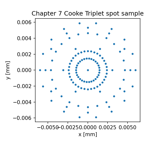
When those rays land on the image plane, their transverse coordinates become data. Plot those coordinates, and you get a spot diagram.
That sentence is the core of this chapter:
A spot diagram is not drawn by hand. It is the plotted landing positions of traced rays.
This sounds obvious once stated. But it is worth making explicit, because spot diagrams are often encountered as finished software plots. The learner sees dots. The software hides the ray generation, the pupil sampling, the surface interactions, and the image-plane intercepts.
Here we will not hide them.
We will build the bundle ourselves.
What a spot diagram really contains
A spot diagram is a scatter plot of ray intersections at an image surface.
For each ray that survives the optical system, we record:
x_image
y_image
Then we plot those points.
If the lens were perfect under geometric optics, rays from one object point would land at one image point. The spot would collapse to a point. Real lenses do not do that. Rays from different parts of the pupil land in slightly different places because of aberrations, defocus, field effects, and wavelength effects.
The spot diagram therefore answers a concrete question:
For this field point,
at this wavelength or wavelength set,
through this aperture,
where do sampled rays land on the image plane?
That question has several hidden inputs:
field point
pupil sampling pattern
aperture size
wavelengths
image plane position
lens prescription
material model
ray tracing algorithm
If you do not know those inputs, the plot is hard to interpret.
A tight spot usually suggests good geometric imaging at that field and wavelength. A wide spot suggests blur. A spot stretched in one direction may suggest astigmatism, coma, field effects, or defocus, depending on context. A spot with different colors separated from each other suggests chromatic aberration.
But the plot itself is not the cause. It is the result.
The computation is:
generate rays
→ trace rays through the optical system
→ collect image-plane intercepts
→ plot intercepts
That is what we will build.
From aperture to pupil sampling
To generate a bundle, we need to decide where rays enter the system.
For a simple object-at-infinity example, all rays from one field point enter with the same direction. The rays differ by where they pass through the entrance pupil or, in our simplified early model, where they start on a launch plane before the lens.
Let us start with a normalized pupil coordinate:
(px, py)
where the circular pupil is:
px² + py² <= 1
If the physical pupil radius is R_pupil, then the ray starting coordinates can be:
x = R_pupil px
y = R_pupil py
This gives us a set of ray starting positions across a circular aperture.
There are many ways to sample a pupil:
square grid clipped to a circle
polar grid
rings and spokes
random sampling
quasi-random sampling
Gaussian quadrature
For this chapter, we will use a square grid clipped to a circle. It is not the most elegant sampling method, but it is easy to inspect. That matters more right now.
Here is the function:
import numpy as np

def sample_pupil_grid(samples_per_axis, pupil_radius):
    """Return pupil sample points on a square grid clipped to a circle.

    Parameters
    ----------
    samples_per_axis:
        Number of grid points along x and y before circular clipping.

    pupil_radius:
        Physical pupil radius in the same length unit as the lens, usually mm.

    Returns
    -------
    An array of shape (N, 2), containing x, y pupil coordinates.
    """
    coords = np.linspace(-pupil_radius, pupil_radius, samples_per_axis)
    points = []

    for x in coords:
        for y in coords:
            if x*x + y*y <= pupil_radius*pupil_radius:
                points.append((x, y))

    return np.array(points, dtype=float)
Test it:
pupil_points = sample_pupil_grid(samples_per_axis=9, pupil_radius=5.0)
print(pupil_points.shape)
print(pupil_points[:5])
This gives a set of points inside a circular aperture of radius 5 mm.
Plot the samples:
import matplotlib.pyplot as plt

plt.scatter(pupil_points[:, 0], pupil_points[:, 1])
plt.gca().set_aspect("equal", adjustable="box")
plt.xlabel("pupil x [mm]")
plt.ylabel("pupil y [mm]")
plt.title("Square-grid pupil sampling clipped to a circle")
plt.show()
This plot is not a spot diagram. It is the input sampling pattern.
That distinction matters.
The pupil plot shows where rays enter the aperture. The spot diagram shows where those rays land after tracing.
Field sampling: where the object point is
A pupil sample tells us where a ray passes through the aperture.
A field point tells us which object point the ray comes from.
For an object at infinity, a field can be represented by an incoming angle. An on-axis field has rays traveling along the optical axis:
θx = 0
θy = 0
An off-axis field may have rays tilted by a few degrees:
θx = 0
θy = 5 degrees
or, depending on coordinate convention, field may be represented in x or y. We will keep a simple two-angle model:
theta_x_deg
theta_y_deg
The direction helper from Chapter 4 was:
import math

def normalize(v):
    v = np.asarray(v, dtype=float)
    norm = np.linalg.norm(v)

    if norm == 0:
        raise ValueError("Cannot normalize a zero vector.")

    return v / norm

def direction_from_field_angles(theta_x_deg=0.0, theta_y_deg=0.0):
    """Create a ray direction from field angles.

    The ray points toward (tan θx, tan θy, 1).
    This is a convenient object-at-infinity model.
    """
    tx = math.tan(math.radians(theta_x_deg))
    ty = math.tan(math.radians(theta_y_deg))
    return normalize([tx, ty, 1.0])
For a given field point, all rays in the bundle share this direction. They start from different pupil coordinates, but they are parallel.
That is the object-at-infinity approximation:
same field → same incoming direction
different pupil coordinates → different ray starting positions
This is not the only possible object model. For a finite object, rays would originate from a finite object point and pass through different pupil locations. But object-at-infinity is natural for many optical examples, and it keeps the first spot diagram readable.
Making a ray bundle
Now combine field direction and pupil coordinates.
We choose a launch plane before the first surface:
z_start = -20 mm
For each pupil sample (x, y), create a ray:
position = [x, y, z_start]
direction = direction_from_field_angles(theta_x, theta_y)
wavelength = selected wavelength
Here is the code:
def make_ray_bundle(
    pupil_points,
    z_start,
    theta_x_deg=0.0,
    theta_y_deg=0.0,
    wavelength_um=0.5875618,
    intensity=1.0,
):
    """Create a bundle of rays from pupil samples and field angles."""
    direction = direction_from_field_angles(theta_x_deg, theta_y_deg)
    rays = []

    for x, y in pupil_points:
        rays.append(
            Ray(
                position=[x, y, z_start],
                direction=direction,
                wavelength_um=wavelength_um,
                intensity=intensity,
            )
        )

    return rays
Create an on-axis bundle:
pupil_points = sample_pupil_grid(samples_per_axis=11, pupil_radius=5.0)

rays = make_ray_bundle(
    pupil_points=pupil_points,
    z_start=-20.0,
    theta_x_deg=0.0,
    theta_y_deg=0.0,
    wavelength_um=0.5875618,
)

print(len(rays))
print(rays[0].position, rays[0].direction)
Now we have many rays.
They do not yet form a spot diagram. They are only the input bundle.
The next step is to trace each one.
Reusing the singlet tracer
From Chapter 6, we had a simple biconvex singlet:
front = IntersectableSurface(
    radius=50.0,
    z_vertex=0.0,
    semi_diameter=10.0,
    comment="front surface"
)

back = IntersectableSurface(
    radius=-50.0,
    z_vertex=5.0,
    semi_diameter=10.0,
    comment="back surface"
)

image = IntersectableSurface(
    radius=float("inf"),
    z_vertex=50.0,
    semi_diameter=None,
    surface_type="plane",
    comment="image plane"
)
And a tracing function:
def trace_simple_singlet_ray(ray, front, back, image, glass_material):
    n_air = 1.0
    n_glass = glass_material.n(ray.wavelength_um)

    interact_refractive_surface(ray, front, n1=n_air, n2=n_glass)

    if ray.alive:
        interact_refractive_surface(ray, back, n1=n_glass, n2=n_air)

    if ray.alive:
        hit_image = intersect_surface(ray, image)

        if hit_image is None:
            ray.stop("missed image plane")
        else:
            ray.propagate(hit_image.t, refractive_index=n_air)

    return ray
Now apply it to a bundle:
def trace_bundle_through_singlet(rays, front, back, image, glass_material):
    traced = []

    for ray in rays:
        traced.append(
            trace_simple_singlet_ray(
                ray,
                front=front,
                back=back,
                image=image,
                glass_material=glass_material,
            )
        )

    return traced
Trace:
traced_rays = trace_bundle_through_singlet(
    rays,
    front=front,
    back=back,
    image=image,
    glass_material=N_BK7,
)
Now every ray has either reached the image plane or stopped somewhere.
Before plotting, we should collect only the rays that survived.
Collecting image-plane intercepts
A spot diagram needs the image-plane positions of valid rays.
def collect_image_points(traced_rays):
    """Return image-plane x, y points from rays that reached the image plane."""
    points = []
    valid_rays = []

    for ray in traced_rays:
        if ray.alive:
            points.append((ray.position[0], ray.position[1]))
            valid_rays.append(ray)

    return np.array(points, dtype=float), valid_rays
Use it:
spot_points, valid_rays = collect_image_points(traced_rays)

print("traced rays:", len(traced_rays))
print("valid rays:", len(valid_rays))
print("spot points:", spot_points.shape)
This is the raw data behind a spot diagram.
Do not plot yet. First look at the numbers.
print(spot_points[:10])
You should see x and y positions at the image plane.
For an on-axis rotationally symmetric system, the spot should be centered near the axis if the image plane is close to focus. If the image plane is not at best focus, the spot may form a larger blur circle.
That is not a bug. The image plane location is one of the inputs.
Plotting the first spot diagram
Now we can plot.
def plot_spot(points, title="Spot diagram"):
    if len(points) == 0:
        raise ValueError("No valid spot points to plot.")

    plt.scatter(points[:, 0], points[:, 1], s=12)
    plt.axhline(0.0, linewidth=0.5)
    plt.axvline(0.0, linewidth=0.5)
    plt.gca().set_aspect("equal", adjustable="box")
    plt.xlabel("image x [mm]")
    plt.ylabel("image y [mm]")
    plt.title(title)
    plt.show()

plot_spot(spot_points, title="On-axis spot diagram")
There it is.
The plot may be unimpressive at first. It is just dots. Good. We should not rush past that. Those dots are not decorative. They are the final coordinates of rays that were:
generated from pupil samples
propagated to the front surface
refracted into glass
propagated to the back surface
refracted into air
propagated to the image plane
recorded as x, y coordinates
A spot diagram is the visible end of a ray-tracing pipeline.
This is the first real analysis graph we have built from our own computation.
Centered spot diagrams
Many optical software spot diagrams are shown relative to a reference point, such as the chief ray intercept or the centroid of the spot. That makes the shape of the blur easier to inspect.
If the absolute image position is large, the spot may be far from the origin. Centering helps us see the spread.
Two common choices are:
subtract the chief ray intercept
subtract the centroid of all valid ray intercepts
For now, centroid centering is simple:
def center_points_by_centroid(points):
    centroid = points.mean(axis=0)
    return points - centroid, centroid
Use it:
centered_points, centroid = center_points_by_centroid(spot_points)

print("centroid:", centroid)

plot_spot(centered_points, title="On-axis spot diagram, centered by centroid")
The centered plot tells you the spread pattern. The centroid tells you where the whole bundle landed.
Do not confuse these.
Absolute spot position is useful for image location and distortion.
Centered spot shape is useful for blur and aberration inspection.
Both are data. They answer different questions.
Spot size metrics
A spot diagram is visual, but we often want summary numbers.
A simple one is RMS spot radius.
Given image points (x_i, y_i) and a reference center (x_c, y_c), the RMS radius is:
r_rms = sqrt(mean((x_i - x_c)² + (y_i - y_c)²))
In code:
def rms_spot_radius(points, center=None):
    """Compute RMS spot radius around a center."""
    if len(points) == 0:
        return np.nan

    if center is None:
        center = points.mean(axis=0)

    shifted = points - center
    r2 = shifted[:, 0]**2 + shifted[:, 1]**2
    return math.sqrt(float(np.mean(r2)))
Compute it:
rms = rms_spot_radius(spot_points)
print("RMS spot radius [mm]:", rms)
Another simple metric is maximum radius:
def max_spot_radius(points, center=None):
    if len(points) == 0:
        return np.nan

    if center is None:
        center = points.mean(axis=0)

    shifted = points - center
    r = np.sqrt(shifted[:, 0]**2 + shifted[:, 1]**2)
    return float(np.max(r))

print("Max spot radius [mm]:", max_spot_radius(spot_points))
These numbers are not replacements for understanding. They are summaries. They tell you how large the traced spot is under the chosen conditions.
Always remember the hidden conditions:
which field
which wavelength
which aperture
which image plane
which pupil sampling
Without those, an RMS spot radius is just a number floating in space.
Chief ray and marginal ray
Now we need two important ray names.
The chief ray is the ray from a field point that passes through the center of the aperture stop.
The marginal ray is often the ray from an on-axis object point that passes through the edge of the aperture stop.
These definitions are simple in words, but they become subtle in real systems because the entrance pupil may not be physically located at the stop surface, especially in multi-element systems. For this chapter’s simplified object-at-infinity model, we can use a practical approximation:
chief ray:
    pupil coordinate near (0, 0) for the selected field

marginal ray:
    pupil coordinate near the edge of the pupil for the on-axis field
This is enough to learn the computational role.
The chief ray helps define image height for an off-axis field. It is often used as a reference for centering spot diagrams.
The marginal ray helps define aperture behavior and first-order quantities. It tells us how an edge ray behaves.
Let us create them in our simple model.
def make_chief_ray(z_start, theta_x_deg=0.0, theta_y_deg=0.0, wavelength_um=0.5875618):
    """Simplified chief ray: starts at pupil center."""
    return Ray(
        position=[0.0, 0.0, z_start],
        direction=direction_from_field_angles(theta_x_deg, theta_y_deg),
        wavelength_um=wavelength_um,
    )

def make_marginal_ray(z_start, pupil_radius, wavelength_um=0.5875618):
    """Simplified marginal ray for an on-axis field: starts at pupil edge."""
    return Ray(
        position=[pupil_radius, 0.0, z_start],
        direction=direction_from_field_angles(0.0, 0.0),
        wavelength_um=wavelength_um,
    )
Trace them:
chief = make_chief_ray(z_start=-20.0, theta_x_deg=0.0, theta_y_deg=3.0)
marginal = make_marginal_ray(z_start=-20.0, pupil_radius=5.0)

trace_simple_singlet_ray(chief, front, back, image, N_BK7)
trace_simple_singlet_ray(marginal, front, back, image, N_BK7)

print("chief image point:", chief.position)
print("marginal image point:", marginal.position)
In a real design program, chief and marginal ray aiming may be more sophisticated. The program may solve for rays that pass through pupil centers and aperture edges after accounting for the optical system before the stop.
But the idea remains:
chief ray → field reference
marginal ray → aperture edge reference
They are special samples inside the larger ray bundle.
Off-axis field spot diagram
Now let us generate a spot for an off-axis field.
For example:
theta_y = 3 degrees
This means all rays enter tilted in the y-z plane. In our simple model, the bundle starts across the pupil and travels with the same tilted direction.
pupil_points = sample_pupil_grid(samples_per_axis=13, pupil_radius=5.0)

off_axis_rays = make_ray_bundle(
    pupil_points=pupil_points,
    z_start=-20.0,
    theta_x_deg=0.0,
    theta_y_deg=3.0,
    wavelength_um=0.5875618,
)

traced_off_axis = trace_bundle_through_singlet(
    off_axis_rays,
    front=front,
    back=back,
    image=image,
    glass_material=N_BK7,
)

off_axis_points, valid_off_axis = collect_image_points(traced_off_axis)

plot_spot(off_axis_points, title="Off-axis spot diagram, absolute coordinates")
The spot may be shifted away from the origin because the field is off-axis. That shift is expected. It is the image height.
To inspect blur shape, center it:
off_axis_centered, off_axis_centroid = center_points_by_centroid(off_axis_points)

print("off-axis centroid:", off_axis_centroid)
print("off-axis RMS radius:", rms_spot_radius(off_axis_points))

plot_spot(off_axis_centered, title="Off-axis spot diagram, centered")
The shape may no longer be circular. It may stretch, skew, or form a pattern that hints at off-axis aberrations.
Do not over-diagnose yet. We have not introduced coma, astigmatism, field curvature, or distortion formally. Chapter 9 will do that. For now, it is enough to see that off-axis ray bundles do not necessarily behave like on-axis bundles.
The spot diagram gives us the evidence.
Field series: center to edge
Optical software often shows spot diagrams for several field points. That lets you see how image quality changes from the center to the edge of the field.
We can do a small version.
def spot_for_field(theta_y_deg, samples_per_axis=13, pupil_radius=5.0, wavelength_um=0.5875618):
    pupil_points = sample_pupil_grid(samples_per_axis, pupil_radius)

    rays = make_ray_bundle(
        pupil_points=pupil_points,
        z_start=-20.0,
        theta_x_deg=0.0,
        theta_y_deg=theta_y_deg,
        wavelength_um=wavelength_um,
    )

    traced = trace_bundle_through_singlet(rays, front, back, image, N_BK7)
    points, valid = collect_image_points(traced)

    return points, valid

for field_angle in [0.0, 1.5, 3.0, 5.0]:
    points, valid = spot_for_field(field_angle)
    centered, centroid = center_points_by_centroid(points)

    print(
        f"field {field_angle:.1f} deg: "
        f"valid rays={len(valid)}, "
        f"centroid={centroid}, "
        f"RMS={rms_spot_radius(points):.6f} mm"
    )
This is already an optical analysis table.
It tells us, under our simplified setup, how the traced spot changes with field angle.
We can plot each field separately. For the book text, separate plots are often clearer than cramming many fields into one graph. Here is one field at a time:
field_angle = 5.0
points, valid = spot_for_field(field_angle)
centered, centroid = center_points_by_centroid(points)

plot_spot(centered, title=f"Centered spot diagram, field = {field_angle} deg")
This pattern is exactly what commercial software automates. But now we know the data pipeline.
Polychromatic ray bundles
So far, we have traced one wavelength at a time.
A real visible-light spot diagram may include multiple wavelengths. Each wavelength uses its own refractive index through the material model. If the plot colors the rays by wavelength, chromatic separation becomes visible.
Let us create a multi-wavelength bundle.
def make_polychromatic_bundle(
    pupil_points,
    z_start,
    theta_x_deg=0.0,
    theta_y_deg=0.0,
    wavelengths_um=(0.4861327, 0.5875618, 0.6562725),
):
    rays = []

    for wl in wavelengths_um:
        rays.extend(
            make_ray_bundle(
                pupil_points=pupil_points,
                z_start=z_start,
                theta_x_deg=theta_x_deg,
                theta_y_deg=theta_y_deg,
                wavelength_um=wl,
            )
        )

    return rays
Trace:
wavelengths = [0.4861327, 0.5875618, 0.6562725]
pupil_points = sample_pupil_grid(samples_per_axis=11, pupil_radius=5.0)

poly_rays = make_polychromatic_bundle(
    pupil_points=pupil_points,
    z_start=-20.0,
    theta_x_deg=0.0,
    theta_y_deg=0.0,
    wavelengths_um=wavelengths,
)

traced_poly = trace_bundle_through_singlet(poly_rays, front, back, image, N_BK7)
Collect points by wavelength:
def collect_points_by_wavelength(traced_rays):
    groups = {}

    for ray in traced_rays:
        if not ray.alive:
            continue

        wl = ray.wavelength_um
        groups.setdefault(wl, []).append((ray.position[0], ray.position[1]))

    return {wl: np.array(points, dtype=float) for wl, points in groups.items()}
Plot:
groups = collect_points_by_wavelength(traced_poly)

for wl, points in groups.items():
    plt.scatter(points[:, 0], points[:, 1], s=12, label=f"{wl:.4f} µm")

plt.gca().set_aspect("equal", adjustable="box")
plt.xlabel("image x [mm]")
plt.ylabel("image y [mm]")
plt.title("Polychromatic spot diagram")
plt.legend()
plt.show()
This plot may show small wavelength-dependent shifts or spread differences. The exact appearance depends on the lens, aperture, field, and image plane.
The important part is not whether this simple singlet gives a beautiful pattern. It will not. The important part is that chromatic behavior has entered through the computation:
ray.wavelength_um
→ material.n(wavelength)
→ different refraction angles
→ different image-plane intercepts
A polychromatic spot diagram is not magic. It is many monochromatic ray traces plotted together or combined according to a defined rule.
Why the spot changes when the image plane moves
A spot diagram is always tied to an image plane position.
Move the image plane, and the same outgoing rays intersect it at different locations. Near focus, the spot may be small. Before or after focus, the spot may expand.
This is not a display setting. It is geometry.
Let us compute RMS spot radius for different image plane positions.
def rms_for_image_plane(z_image, field_angle=0.0, wavelength_um=0.5875618):
    image_surface = IntersectableSurface(
        radius=float("inf"),
        z_vertex=z_image,
        semi_diameter=None,
        surface_type="plane",
        comment="image plane",
    )

    pupil_points = sample_pupil_grid(samples_per_axis=13, pupil_radius=5.0)

    rays = make_ray_bundle(
        pupil_points=pupil_points,
        z_start=-20.0,
        theta_x_deg=0.0,
        theta_y_deg=field_angle,
        wavelength_um=wavelength_um,
    )

    traced = trace_bundle_through_singlet(
        rays,
        front=front,
        back=back,
        image=image_surface,
        glass_material=N_BK7,
    )

    points, valid = collect_image_points(traced)

    if len(points) == 0:
        return np.nan

    return rms_spot_radius(points)
Sweep focus:
z_values = np.linspace(35.0, 65.0, 61)
rms_values = [rms_for_image_plane(z) for z in z_values]

plt.plot(z_values, rms_values)
plt.xlabel("image plane z [mm]")
plt.ylabel("RMS spot radius [mm]")
plt.title("RMS spot radius versus image plane position")
plt.show()
This plot is not a spot diagram. It is a focus scan based on spot size.
The minimum suggests a best-focus region according to our chosen RMS criterion.
This is another important software-output lesson:
A spot diagram depends on focus position. A bad-looking spot may mean the lens is bad, or it may mean the image plane is not placed where that analysis expects.
A real optical program may offer several focus definitions. We will study paraxial focus and first-order quantities in Chapter 8, then aberration and best focus more carefully in Chapter 9.
For now, just remember that the image plane is part of the analysis, not an afterthought.
Pupil sampling density changes the plot
A spot diagram with 9 rays and a spot diagram with 169 rays may show the same system, but they will look different.
The underlying optical system has not changed. The sampling has changed.
Let us compare:
for n in [5, 9, 17]:
    pupil_points = sample_pupil_grid(samples_per_axis=n, pupil_radius=5.0)

    rays = make_ray_bundle(
        pupil_points=pupil_points,
        z_start=-20.0,
        theta_y_deg=3.0,
        wavelength_um=0.5875618,
    )

    traced = trace_bundle_through_singlet(rays, front, back, image, N_BK7)
    points, valid = collect_image_points(traced)
    centered, centroid = center_points_by_centroid(points)

    print(
        f"samples_per_axis={n}, "
        f"valid rays={len(valid)}, "
        f"RMS={rms_spot_radius(points):.6f} mm"
    )

    plot_spot(centered, title=f"Centered spot, field 3 deg, grid {n}x{n}")
The rough shape should become clearer as sampling density increases. But more samples also cost more computation.
This is a small preview of a major theme in computational optics:
sampling choices affect numerical results and visual interpretation
We will revisit this forcefully in Chapter 14 when we discuss sampling, normalization, and FFT grids. For spot diagrams, the stakes are already visible. A sparse spot can hide structure. A dense spot can reveal it. A poorly chosen pattern can mislead.
The plot is only as honest as the sampling behind it.
A better pupil sampler: rings and angles
A square grid clipped to a circle is easy, but optical ray diagrams often use ring-based sampling. That gives more direct control over radial positions.
Here is a simple polar sampler:
def sample_pupil_polar(num_rings, points_per_ring, pupil_radius, include_center=True):
    """Return pupil points sampled on concentric rings."""
    points = []

    if include_center:
        points.append((0.0, 0.0))

    for ring in range(1, num_rings + 1):
        r = pupil_radius * ring / num_rings
        count = points_per_ring * ring

        for j in range(count):
            phi = 2.0 * math.pi * j / count
            x = r * math.cos(phi)
            y = r * math.sin(phi)
            points.append((x, y))

    return np.array(points, dtype=float)
Plot it:
polar_points = sample_pupil_polar(
    num_rings=4,
    points_per_ring=6,
    pupil_radius=5.0
)

plt.scatter(polar_points[:, 0], polar_points[:, 1])
plt.gca().set_aspect("equal", adjustable="box")
plt.xlabel("pupil x [mm]")
plt.ylabel("pupil y [mm]")
plt.title("Polar pupil sampling")
plt.show()
Now trace it:
rays = make_ray_bundle(
    pupil_points=polar_points,
    z_start=-20.0,
    theta_y_deg=3.0,
    wavelength_um=0.5875618,
)

traced = trace_bundle_through_singlet(rays, front, back, image, N_BK7)
points, valid = collect_image_points(traced)
centered, centroid = center_points_by_centroid(points)

plot_spot(centered, title="Centered spot from polar pupil sampling")
The spot may look different from the square-grid version because the pupil samples are different. The lens did not change. The sampling changed.
That is an important lesson. A spot diagram is a sampled view of ray behavior, not the continuous truth itself.
Vignetting and blocked rays
Not every generated ray necessarily reaches the image plane.
A ray may be stopped because:
it misses a surface
it hits outside a clear aperture
it undergoes total internal reflection
it fails to reach the image plane
For a spot diagram, we normally plot only rays that survive to the image plane. But we should also count the lost rays.
def ray_status_counts(rays):
    counts = {}

    for ray in rays:
        key = "alive" if ray.alive else ray.stop_reason
        counts[key] = counts.get(key, 0) + 1

    return counts
Use it:
counts = ray_status_counts(traced)
print(counts)
If many rays are blocked, the spot diagram alone may not tell the whole story. A tiny spot made from a few surviving rays is not automatically good news. It may mean most of the aperture is being clipped.
This is why optical software often reports vignetting or ray failures separately.
The spot diagram answers:
Where did surviving rays land?
It does not fully answer:
How many rays failed to get there?
You need both.
Reading a spot diagram carefully
A spot diagram can tell you many things, but it can also tempt you to overread.
Here is a careful way to read it.
First, check the conditions:
field point
wavelength or wavelength set
aperture
image plane position
sampling pattern
reference center
units
Second, look at the scale. A spot that looks large on a plot may be tiny in millimeters. A spot that looks small may still be large compared with pixel size or diffraction scale.
Third, ask whether the plot is absolute or centered. Absolute coordinates show image location. Centered coordinates show spread.
Fourth, check whether all rays survived. A clean spot from a heavily clipped bundle can be misleading.
Fifth, compare across fields and wavelengths. A lens may be good on-axis and poor off-axis. It may be good in green and worse in blue or red.
Sixth, remember the limitation:
A geometric spot diagram does not include diffraction.
That last point matters.
A perfect geometric spot can still produce a finite diffraction pattern. Conversely, a small geometric spot does not automatically mean excellent MTF at every spatial frequency. Spot diagrams are useful, but they are not the whole imaging story.
This book is moving toward PSF and MTF precisely because geometric ray landing points are not enough.
But for now, spot diagrams are the right next step. They show what real rays do.
Spot diagram versus ray fan
It is useful to distinguish two common ray-based plots.
A spot diagram plots image-plane landing points:
x_image, y_image
A ray fan plot usually plots transverse ray error versus pupil coordinate:
pupil coordinate → ray error
Both are built from traced rays. They simply organize the results differently.
Spot diagram asks:
Where did the rays land?
Ray fan asks:
How does the landing error vary across the pupil?
Chapter 9 will use ray fans to discuss aberrations more clearly. For now, the spot diagram is the simpler visual result.
But keep the relationship in mind:
same traced rays
different plotted quantities
That is a recurring pattern in optical analysis.
Optiland SpotDiagram comparison
Now let us compare our teaching pipeline with a real library-level call.
In Optiland, the high-level workflow is much shorter. After building or loading an optical system, a spot diagram can be generated through an analysis object.
A compact example looks like this:
from optiland.samples.objectives import CookeTriplet
from optiland.analysis import SpotDiagram

lens = CookeTriplet()

spot = SpotDiagram(lens)
spot.view()
For a custom singlet, the workflow follows the same spirit:
from optiland import optic
from optiland.analysis import SpotDiagram

lens = optic.Optic()

lens.surfaces.add(index=0, radius=float("inf"), thickness=float("inf"))
lens.surfaces.add(index=1, radius=50.0, thickness=5.0, material="N-BK7", is_stop=True)
lens.surfaces.add(index=2, radius=-50.0, thickness=45.0)
lens.surfaces.add(index=3)

lens.set_aperture(aperture_type="EPD", value=10.0)
lens.fields.set_type("angle")
lens.fields.add(y=0.0)
lens.fields.add(y=3.0)
lens.wavelengths.add(value=0.5876, is_primary=True)

spot = SpotDiagram(lens)
spot.view()
Exact options and method signatures may vary by version, so treat this as the conceptual comparison rather than a promise about every installed environment.
The important point is what the library call hides.
When you call:
spot = SpotDiagram(lens)
spot.view()
the library must do some version of this:
read fields
read wavelengths
read aperture definition
generate ray samples
trace rays through all surfaces
collect image-plane intercepts
plot the points
That is the same pipeline we built manually.
The difference is that Optiland provides the full framework, better surface handling, proper system bookkeeping, and analysis tools. Our code is a teaching skeleton. It exists to make the calculation visible.
We are not replacing the library. We are identifying the calculations the library performs when the plot appears.
Why our plot may not match Optiland exactly
If you compare our spot diagram with Optiland’s and they differ, do not panic.
There are many possible reasons:
different pupil sampling
different ray aiming
different aperture definition
different image plane handling
different material data
different wavelength convention
different field coordinate convention
different focus solve
different normalization or centering
This is not a failure of the comparison. It is part of the lesson.
Optical analysis is full of conventions. A spot diagram is not just “the spot diagram.” It is a spot diagram under specified conditions.
To make a fair comparison, you must match:
lens prescription
surface signs
glass model
wavelengths
aperture type and value
field type and value
image surface position
ray sampling pattern
plot centering convention
That is a lot. It is also exactly why understanding the computation matters.
If all you have is the final plot, you may not know which convention caused the difference.
If you understand the pipeline, you know where to look.
A compact bundle trace summary
Let us gather the chapter’s essential code path in one place.
# 1. Choose pupil sampling.
pupil_points = sample_pupil_grid(samples_per_axis=13, pupil_radius=5.0)

# 2. Choose field and wavelength.
theta_y_deg = 3.0
wavelength_um = 0.5875618

# 3. Generate rays.
rays = make_ray_bundle(
    pupil_points=pupil_points,
    z_start=-20.0,
    theta_x_deg=0.0,
    theta_y_deg=theta_y_deg,
    wavelength_um=wavelength_um,
)

# 4. Trace rays.
traced_rays = trace_bundle_through_singlet(
    rays,
    front=front,
    back=back,
    image=image,
    glass_material=N_BK7,
)

# 5. Collect image-plane intercepts.
spot_points, valid_rays = collect_image_points(traced_rays)

# 6. Center and summarize.
centered_points, centroid = center_points_by_centroid(spot_points)
rms_radius = rms_spot_radius(spot_points)

print("valid rays:", len(valid_rays))
print("centroid:", centroid)
print("RMS spot radius:", rms_radius)

# 7. Plot.
plot_spot(centered_points, title="Centered spot diagram")
This is the entire spot diagram pipeline in miniature.
It is short because the earlier chapters have already done their work.
That is the pleasure of building the chain carefully. Once the pieces are in place, the analysis function is not mysterious.
What this chapter adds to the full computation chain
At the beginning of the book, the chain was:
lens prescription
→ surfaces and materials
→ real ray tracing
→ paraxial reference
→ pupil sampling
→ optical path difference
→ pupil function
→ point spread function
→ optical transfer function
→ modulation transfer function
This chapter fills in a crucial part of “real ray tracing” and introduces pupil sampling as a deliberate computational action.
We can now say:
lens prescription defines surfaces
material model defines n(λ)
ray object carries position, direction, and wavelength
intersection finds hit points
vector Snell computes new directions
pupil sampling generates many rays
field sampling sets incoming direction
image-plane intercepts produce spot diagrams
That is a real computational path from data to plot.
No MTF yet. No PSF yet. No wavefront yet. But the foundation is no longer abstract.
You can generate rays, trace them, and plot where they land.
That is one of the first moments when optical software begins to feel less like an oracle and more like a collection of understandable algorithms.
Common mistakes when generating ray bundles
Let us collect the traps.
Mistake 1: Confusing pupil plot with spot plot
The pupil plot shows where rays start or pass through the aperture.
The spot plot shows where traced rays land on the image plane.
They are not the same plot.
Mistake 2: Forgetting the field direction
For an object at infinity, different field points mean different incoming directions. If every bundle uses the same direction, you are only testing one field.
Mistake 3: Comparing spot diagrams with different sampling
A 5-by-5 pupil grid and a 21-by-21 pupil grid may show different visual structure. Match sampling before comparing plots.
Mistake 4: Ignoring blocked rays
A spot diagram of surviving rays should be read together with ray failure counts. A small spot after severe clipping can be misleading.
Mistake 5: Forgetting image plane position
Move the image plane, and the spot changes. A large spot may indicate defocus, not only aberration.
Mistake 6: Mixing absolute and centered coordinates
Absolute spot plots show image position. Centered plots show spread. Know which one you are looking at.
Mistake 7: Treating spot diagrams as diffraction results
Spot diagrams are geometric ray results. They do not show diffraction blur. They are important, but they are not PSF or MTF.
Mistake 8: Calling the chief ray “the center ray” without field context
For a simple on-axis setup, the chief ray may look like the central ray. For off-axis fields and real pupil definitions, chief ray meaning is tied to the aperture stop and field point.
Mistake 9: Over-interpreting a simple teaching lens
Our singlet is a learning system. It is not optimized. If the spots look ugly, that may be the correct result.
The purpose here is to understand the computation, not to pretend a simple biconvex lens is a modern imaging objective.
What you should be able to do now
You should now be able to explain a spot diagram without saying:
The software draws it.
A better answer is:
The program samples rays across the pupil for a selected field and wavelength, traces those rays through the lens using ray-surface intersections and Snell refraction, records where the surviving rays hit the image plane, and plots those intercepts.
That sentence contains the whole chapter.
You should also be able to identify the main inputs:
pupil sampling
field angle
wavelength
aperture
image plane
lens prescription
material model
And you should be able to write a minimal Python version that produces the plot.
That is a meaningful milestone.
The road ahead
We have now completed the first working version of real ray tracing.
But real ray tracing alone is not enough to understand an optical system.
In the next chapter, we will deliberately step backward into approximation.
That may sound strange. After working so hard to trace real rays, why go back to paraxial optics?
Because paraxial optics gives us the skeleton of the system.
Real rays show what actually happens. Paraxial rays show the first-order structure: focal length, image position, F-number, magnification, and principal behavior near the axis.
Without that skeleton, spot diagrams can become isolated pictures. You may see that rays spread, but not know what they are spreading around. You may see that focus changes, but not know the first-order focus reference. You may trace many rays, but not know the system’s basic optical power.
So Chapter 8 will introduce paraxial optics not as an old-fashioned detour, but as the coordinate system of understanding.
The real-ray tracer tells us where rays actually go.
Paraxial optics tells us what the system was trying to do in the first place.
Generated validation figure