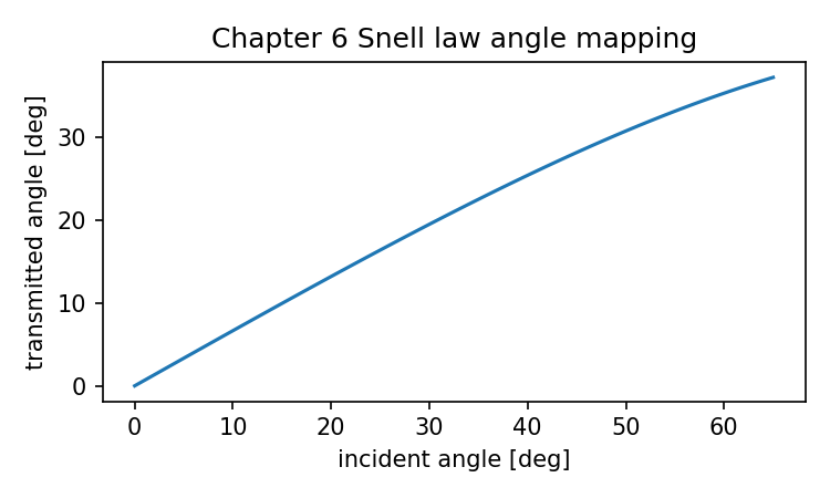
Chapter 6: How Refraction Direction Is Computed
A ray has now reached the surface.
That sentence sounds simple only because we have already done the hidden work.
In Chapter 4, we gave the ray a position, a direction, a wavelength, an intensity, and an optical path length. In Chapter 5, we made that ray collide with a plane or spherical surface. We computed the hit point. We checked the clear aperture. We computed the local surface normal.
Now the ray is sitting at the surface.
It has an incoming direction:
d_in
The surface has a local normal:
N
The material model gives refractive indices on the two sides:
n1 = refractive index before the surface
n2 = refractive index after the surface
The next question is the one every optics student expects:
In what direction does the ray go after refraction?
This chapter answers that question.
We will begin with scalar Snell’s law, but we will not stay there. Optical software does not usually trace rays by drawing angles with a protractor. It has direction vectors and surface normals. So the useful form is vector refraction.
That is where many errors happen.
The formula itself is not very long. The hard parts are:
normal direction
unit vectors
which index is n1 and which is n2
total internal reflection
numerical tolerance
We will go slowly. This is one of the load-bearing chapters of the book.
After this chapter, the ray will finally do what lens drawings have shown all along:
hit a surface
bend according to the local normal and refractive indices
continue in a new direction
Only now, the bending will be computed.
Start with scalar Snell’s law
The familiar form of Snell’s law is:
n1 sin θ1 = n2 sin θ2
where:
n1 = refractive index of the incident medium
n2 = refractive index of the transmitted medium
θ1 = incident angle measured from the surface normal
θ2 = refracted angle measured from the surface normal
This law says that the ray changes direction when it crosses between media with different refractive indices.
If light goes from air into glass:
n1 ≈ 1.0
n2 ≈ 1.5
then the ray bends toward the normal.
If light goes from glass into air:
n1 ≈ 1.5
n2 ≈ 1.0
then the ray bends away from the normal.
At normal incidence, where θ1 = 0, the ray does not change direction. It may change speed and wavelength inside the medium, but its geometric direction remains the same.
Let us first write a scalar angle function, just to see the law numerically.
import math

def snell_angle(theta1_deg, n1, n2):
    """Return refracted angle in degrees using scalar Snell's law.

    theta1_deg is measured from the surface normal.
    Returns None if total internal reflection occurs.
    """
    theta1 = math.radians(theta1_deg)
    sin_theta2 = (n1 / n2) * math.sin(theta1)

    if abs(sin_theta2) > 1.0:
        return None

    theta2 = math.asin(sin_theta2)
    return math.degrees(theta2)
Try air to glass:
for theta in [0, 10, 20, 30, 40]:
    theta2 = snell_angle(theta, n1=1.0, n2=1.5)
    print(theta, "→", theta2)
The refracted angles are smaller. The ray bends toward the normal.
Try glass to air:
for theta in [0, 10, 20, 30, 40, 50]:
    theta2 = snell_angle(theta, n1=1.5, n2=1.0)
    print(theta, "→", theta2)
At some incident angle, the function returns None. That is total internal reflection.
The scalar form is useful for intuition. But it is not enough for real ray tracing.
A ray tracer does not usually store “angle from normal.” It stores:
incoming direction vector
surface normal vector
So we need the vector version.
Why scalar angles are not enough
Imagine a ray hitting a spherical surface away from the optical axis.
The local normal is not [0, 0, 1]. It points outward from the sphere center through the hit point. Its x and y components may be nonzero.
In scalar Snell’s law, you can say:
the incident angle is θ1
the refracted angle is θ2
But in three-dimensional code, that does not tell you the outgoing vector. There are infinitely many directions that make the same angle with a normal unless you also know the plane of incidence.
The plane of incidence is defined by:
incoming direction
surface normal
The refracted ray must stay in that plane. A vector formula handles this automatically.
So the computational task is:
given:
    d_in, normal, n1, n2

compute:
    d_out
where both direction vectors are unit length.
That is the function we want:
d_out = refract_direction(d_in, normal, n1, n2)
But before writing it, we must handle a surprisingly important detail.
The normal has two possible directions
A surface normal can point in either of two opposite directions.
For a plane, both of these are valid normals:
[0, 0, 1]
[0, 0, -1]
For a sphere, the geometric normal often points outward from the sphere center. That is a perfectly good geometric normal. But for refraction, the formula needs the normal to be oriented consistently relative to the incoming ray.
This is where many ray tracers first go wrong.
Let us define a convention:
Before applying the vector refraction formula, orient the normal so that it points against the incoming ray.
In other words, after orientation:
dot(d_in, normal) <= 0
If the incoming ray points roughly in +z, the oriented normal should point roughly back toward the incident side.
Here is the helper function:
import numpy as np

def normalize(v):
    """Return a unit-length copy of vector v."""
    v = np.asarray(v, dtype=float)
    norm = np.linalg.norm(v)

    if norm == 0:
        raise ValueError("Cannot normalize a zero vector.")

    return v / norm

def orient_normal_against_ray(direction, normal):
    """Orient normal so that it points against the incoming direction."""
    d = normalize(direction)
    n = normalize(normal)

    if np.dot(d, n) > 0:
        n = -n

    return n
Test it:
d_in = np.array([0.0, 0.0, 1.0])

print(orient_normal_against_ray(d_in, [0, 0, 1]))
print(orient_normal_against_ray(d_in, [0, 0, -1]))
Both cases should produce:
[ 0. 0. -1.]
That is what we want. The refraction function should not care whether the surface gave us [0,0,1] or [0,0,-1]. It should orient the normal before using it.
This small function removes a large class of sign bugs.
The vector refraction formula
Let:
i = incoming unit direction
n = unit normal oriented against the incoming ray
η = n1 / n2
The cosine of the incident angle is:
cosθ1 = - i · n
The transmitted direction can be written as:
t = η i + (η cosθ1 - cosθ2) n
where:
cosθ2 = sqrt(1 - η²(1 - cos²θ1))
The term under the square root is important:
k = 1 - η²(1 - cos²θ1)
If k < 0, there is no real refracted ray. That is total internal reflection.
This is the complete computational logic.
normalize incoming direction
normalize and orient normal
compute η = n1 / n2
compute cosθ1
compute k
if k < 0: total internal reflection
else compute outgoing direction
normalize outgoing direction
Now write it in Python.
def refract_direction(direction, normal, n1, n2, eps=1e-12):
    """Compute refracted ray direction using vector Snell's law.

    Parameters
    ----------
    direction:
        Incoming ray direction. It does not need to be pre-normalized.

    normal:
        Surface normal at the hit point. It may point either way;
        this function orients it against the incoming ray.

    n1:
        Refractive index of the incident medium.

    n2:
        Refractive index of the transmitted medium.

    Returns
    -------
    A unit outgoing direction vector, or None if total internal reflection occurs.
    """
    i = normalize(direction)
    n = orient_normal_against_ray(i, normal)

    eta = n1 / n2
    cos_theta1 = -float(np.dot(i, n))

    # Numerical safety: keep cosine inside valid range.
    cos_theta1 = max(-1.0, min(1.0, cos_theta1))

    sin2_theta2 = eta * eta * (1.0 - cos_theta1 * cos_theta1)

    if sin2_theta2 > 1.0 + eps:
        return None

    # Clamp tiny numerical overshoot.
    sin2_theta2 = min(1.0, max(0.0, sin2_theta2))
    cos_theta2 = math.sqrt(1.0 - sin2_theta2)

    t = eta * i + (eta * cos_theta1 - cos_theta2) * n
    return normalize(t)
This function is the heart of the chapter.
It is not a black box. It is a direct computational form of Snell’s law.
The incoming ray direction and the surface normal define the plane of incidence. The refractive-index ratio controls the bending. The square root test detects total internal reflection.
Now we must test it carefully.
A helper for measuring angles
To compare with scalar Snell’s law, we need a way to measure the angle between a direction and the normal line.
The normal line has two directions, normal and -normal, so we use the absolute value of the dot product.
def angle_to_normal_line(direction, normal):
    """Return the smaller angle between a direction and the normal line."""
    d = normalize(direction)
    n = normalize(normal)
    c = abs(float(np.dot(d, n)))
    c = max(-1.0, min(1.0, c))
    return math.degrees(math.acos(c))
Now we can test vector refraction against scalar Snell’s law.
Test 1: normal incidence
A ray traveling along the normal should not change direction.
d_in = np.array([0.0, 0.0, 1.0])
normal = np.array([0.0, 0.0, -1.0])

d_out = refract_direction(d_in, normal, n1=1.0, n2=1.5)

print("incoming:", d_in)
print("outgoing:", d_out)
print("angle:", angle_to_normal_line(d_out, normal))
The outgoing direction should still be:
[0, 0, 1]
The angle to the normal line should be 0.
This is a basic sanity check. If this fails, do not continue. Fix the normal orientation or formula first.
Test 2: air to glass
Now use a ray 30 degrees from the normal. Let the normal line be the z axis, and let the ray travel in the x-z plane.
def direction_from_angle_to_z(theta_deg):
    """Direction in x-z plane, traveling generally in +z."""
    theta = math.radians(theta_deg)
    return normalize([math.sin(theta), 0.0, math.cos(theta)])

d_in = direction_from_angle_to_z(30.0)
normal = np.array([0.0, 0.0, -1.0])

d_out = refract_direction(d_in, normal, n1=1.0, n2=1.5)

print("incoming angle:", angle_to_normal_line(d_in, normal))
print("outgoing angle:", angle_to_normal_line(d_out, normal))
print("scalar Snell:", snell_angle(30.0, n1=1.0, n2=1.5))
print("outgoing direction:", d_out)
The vector outgoing angle should match scalar Snell’s law.
Air to glass bends toward the normal, so the outgoing angle should be smaller than 30 degrees.
This test confirms that the vector formula and scalar law agree in a simple plane case.
Test 3: glass to air
Now reverse the indices.
d_in = direction_from_angle_to_z(30.0)
normal = np.array([0.0, 0.0, -1.0])

d_out = refract_direction(d_in, normal, n1=1.5, n2=1.0)

print("incoming angle:", angle_to_normal_line(d_in, normal))
print("outgoing angle:", angle_to_normal_line(d_out, normal))
print("scalar Snell:", snell_angle(30.0, n1=1.5, n2=1.0))
print("outgoing direction:", d_out)
Glass to air bends away from the normal, so the outgoing angle should be larger than 30 degrees.
Again, the vector and scalar results should match.
Test 4: total internal reflection
Total internal reflection occurs when light tries to pass from a higher-index medium to a lower-index medium at too steep an angle.
The critical angle satisfies:
sin θc = n2 / n1
for n1 > n2.
For glass to air:
θc = arcsin(1.0 / 1.5) ≈ 41.8 degrees
So a 50-degree incident angle should not produce a transmitted ray.
d_in = direction_from_angle_to_z(50.0)
normal = np.array([0.0, 0.0, -1.0])

d_out = refract_direction(d_in, normal, n1=1.5, n2=1.0)

print(d_out)
The result should be:
None
That does not mean the ray disappears physically. It means there is no refracted transmitted ray. The interface would reflect the ray internally. In a refractive lens tracing path, we may stop the ray or handle reflection depending on the system model.
For this book’s basic refractive ray tracer, we will stop the ray and record the reason.
Total internal reflection is not an error
It is tempting to treat None as a failure of the code. It is not.
Total internal reflection is a real physical condition. The code is doing its job by detecting that no refracted direction exists.
What the ray tracer does next depends on the optical model.
For a purely refractive system, it may mark the ray invalid:
stop ray: total internal reflection
For a system that supports reflection, it may compute a reflected direction instead:
d_reflect = d_in - 2(d_in · n)n
We will not build a reflective ray tracer here. But it is useful to know that total internal reflection is a branching event, not a numerical accident.
In our basic lens ray tracer, stopping the ray is the right first behavior.
A function for reflection, for comparison
Even though this chapter focuses on refraction, reflection is short enough to show. It also helps clarify normal orientation.
def reflect_direction(direction, normal):
    """Reflect direction across a surface normal."""
    i = normalize(direction)
    n = normalize(normal)

    return normalize(i - 2.0 * np.dot(i, n) * n)
If total internal reflection occurs, a more complete tracer could use this. For now, we will simply stop refractive rays when refraction is impossible.
The main chain of this book is lens imaging, not mirror systems.
Putting wavelength back into the calculation
So far, we have used fixed values like:
n1 = 1.0
n2 = 1.5
But in Chapter 3, we already learned that a real material gives:
n = n(λ)
The ray carries wavelength:
ray.wavelength_um
So at each surface, the tracing code should ask the material library:
n1 = materials.n(material_before, ray.wavelength_um)
n2 = materials.n(material_after, ray.wavelength_um)
That is how chromatic refraction enters the ray tracer.
A blue ray and a red ray may have the same incoming direction and hit the same surface point. But because the glass has different refractive index at different wavelengths, their outgoing directions will differ slightly.
Let us demonstrate this with a plane interface.
Assume we have an N-BK7 material model from Chapter 3:
# N_BK7.n(wavelength_um) returns refractive index.
# For this example, assume N_BK7 is already defined.
Now compare blue, green, and red rays entering glass at 30 degrees.
F_LINE_UM = 0.4861327
D_LINE_UM = 0.5875618
C_LINE_UM = 0.6562725

normal = np.array([0.0, 0.0, -1.0])
d_in = direction_from_angle_to_z(30.0)

for wl in [F_LINE_UM, D_LINE_UM, C_LINE_UM]:
    n_glass = N_BK7.n(wl)
    d_out = refract_direction(d_in, normal, n1=1.0, n2=n_glass)
    angle = angle_to_normal_line(d_out, normal)

    print(f"{wl:.7f} µm  n={n_glass:.7f}  outgoing angle={angle:.6f} deg")
The differences will be small. But they are real.
Shorter wavelengths usually see a higher refractive index in normal dispersion, so the blue ray bends slightly more toward the normal than the red ray.
That is chromatic behavior entering through one line of code:
n_glass = N_BK7.n(wl)
This is why Chapter 3 was not optional. Without wavelength-dependent material indices, a ray tracer cannot show chromatic aberration.
Refraction at a curved surface
Now let us use what Chapter 5 gave us: a hit point and a local normal on a spherical surface.
Imagine a parallel ray entering the front surface of a spherical N-BK7 lens.
We already have:
ray
surface
intersect_surface(ray, surface)
The hit record contains:
hit.point
hit.normal
Now we compute the outgoing direction.
surface = IntersectableSurface(
    radius=50.0,
    z_vertex=0.0,
    semi_diameter=10.0,
    comment="front spherical surface"
)

ray = Ray(
    position=[5.0, 0.0, -20.0],
    direction=[0.0, 0.0, 1.0],
    wavelength_um=0.5875618
)

hit = intersect_surface(ray, surface)

n_air = 1.0
n_glass = N_BK7.n(ray.wavelength_um)

d_out = refract_direction(
    direction=ray.direction,
    normal=hit.normal,
    n1=n_air,
    n2=n_glass
)

print("hit point:", hit.point)
print("surface normal:", hit.normal)
print("incoming direction:", ray.direction)
print("outgoing direction:", d_out)
For an off-axis ray, the surface normal has an x component. The outgoing direction will also gain an x component. That is the surface focusing the ray.
This is the local reason a lens works.
A lens does not “know” where the image plane is. At each surface, the ray only sees:
local normal
incoming direction
index before
index after
The global focusing behavior emerges from many local refractions and propagations.
That is a powerful idea. It is also exactly what ray-tracing software computes.
Updating the ray at the surface
A refraction function returns a direction. But our ray object must actually be updated.
A surface interaction has several steps:
1. find the surface hit
2. propagate the ray to the hit point through the current medium
3. check aperture
4. compute refractive indices
5. compute refracted direction
6. update the ray direction
7. continue into the next medium
Chapters 3, 4, and 5 gave us almost all pieces. Now we combine them.
First, define a small result object:
from dataclasses import dataclass

@dataclass
class RefractionResult:
    success: bool
    direction: np.ndarray | None
    reason: str = ""
If your Python version does not support np.ndarray | None, use Optional[np.ndarray] from typing.
Now wrap the refraction call:
def refract_at_surface(ray, hit, n1, n2):
    """Return a refraction result for a ray at a surface hit."""
    d_out = refract_direction(
        direction=ray.direction,
        normal=hit.normal,
        n1=n1,
        n2=n2
    )

    if d_out is None:
        return RefractionResult(
            success=False,
            direction=None,
            reason="total internal reflection"
        )

    return RefractionResult(
        success=True,
        direction=d_out,
        reason=""
    )
Then a surface interaction can update the ray:
def interact_refractive_surface(ray, surface, n1, n2):
    """Propagate ray to a surface and refract it.

    This function assumes n1 is the index of the medium before the surface
    and n2 is the index after the surface.
    """
    if not ray.alive:
        return None

    hit = intersect_surface(ray, surface)

    if hit is None:
        ray.stop(f"missed surface: {surface.comment}")
        return None

    # Propagate through the incident medium to the hit point.
    ray.propagate(hit.t, refractive_index=n1)

    if not hit.inside_aperture:
        ray.stop(f"blocked by aperture: {surface.comment}")
        return hit

    result = refract_at_surface(ray, hit, n1=n1, n2=n2)

    if not result.success:
        ray.stop(result.reason)
        return hit

    old_direction = ray.direction.copy()
    ray.direction = result.direction

    ray.history.append({
        "event": "refract",
        "surface": surface.comment,
        "point": ray.position.copy(),
        "normal": hit.normal.copy(),
        "n1": n1,
        "n2": n2,
        "direction_before": old_direction,
        "direction_after": ray.direction.copy(),
    })

    return hit
This function is a milestone.
A ray can now:
find a surface
move to the surface
check aperture
bend into the next medium
carry on with a new direction
That is real ray tracing.
Still simple, yes. But real.
Tracing through a single spherical interface
Let us trace a few parallel rays entering a spherical air-to-glass interface.
surface = IntersectableSurface(
    radius=50.0,
    z_vertex=0.0,
    semi_diameter=10.0,
    comment="air-to-glass spherical surface"
)

rays = [
    Ray(position=[x, 0.0, -20.0], direction=[0.0, 0.0, 1.0], wavelength_um=0.5875618)
    for x in np.linspace(-8.0, 8.0, 5)
]

n_air = 1.0
n_glass = N_BK7.n(0.5875618)

for ray in rays:
    interact_refractive_surface(ray, surface, n1=n_air, n2=n_glass)

    print(
        "position:", ray.position,
        "direction:", ray.direction,
        "alive:", ray.alive
    )
The on-axis ray should remain along the z direction. Off-axis rays should bend inward. Rays on opposite sides should bend symmetrically.
This symmetry is a useful sanity check. If both off-axis rays bend in the same transverse direction, something is wrong.
Most likely causes:
normal sign error
surface center sign error
wrong n1/n2 order
incorrect intersection branch
The debugging trail is already clear because we kept the functions separate.
Visualizing the bend
Let us plot incoming and outgoing segments around the spherical surface.
import matplotlib.pyplot as plt

def line_points(start, direction, length):
    start = np.asarray(start, dtype=float)
    direction = normalize(direction)
    end = start + length * direction
    return start, end

surface = IntersectableSurface(
    radius=50.0,
    z_vertex=0.0,
    semi_diameter=10.0,
    comment="front spherical surface"
)

rays = [
    Ray(position=[x, 0.0, -20.0], direction=[0.0, 0.0, 1.0], wavelength_um=0.5875618)
    for x in np.linspace(-8.0, 8.0, 7)
]

plt.figure()

# Draw surface profile in x-z plane.
xs = np.linspace(-10.0, 10.0, 300)
zs = [spherical_sag(x, 0.0, surface) for x in xs]
plt.plot(zs, xs, label="spherical surface")

for ray in rays:
    start = ray.position.copy()
    incoming_dir = ray.direction.copy()

    hit = interact_refractive_surface(ray, surface, n1=1.0, n2=N_BK7.n(ray.wavelength_um))

    if hit is None:
        continue

    hit_point = ray.position.copy()
    outgoing_dir = ray.direction.copy()

    # Incoming segment.
    plt.plot([start[2], hit_point[2]], [start[0], hit_point[0]], linewidth=0.8)

    # Outgoing segment preview.
    end = hit_point + 25.0 * outgoing_dir
    plt.plot([hit_point[2], end[2]], [hit_point[0], end[0]], linewidth=0.8)

plt.xlabel("z [mm]")
plt.ylabel("x [mm]")
plt.title("Refraction at a spherical air-glass surface")
plt.gca().set_aspect("equal", adjustable="box")
plt.legend()
plt.show()
The drawing is now earned.
It is not a decorative sketch. It is a visualization of computed intersections and computed refracted directions.
This is exactly the kind of shift we want throughout the book.
The order of n1 and n2 matters
At the front surface of a lens:
air → glass
so:
n1 = n_air
n2 = n_glass
At the back surface:
glass → air
so:
n1 = n_glass
n2 = n_air
If you reverse them, the ray will bend the wrong way.
This is why the material transition logic from Chapter 3 matters. The tracing code should not guess.
A function like this is helpful:
def material_before_after(lens, surface_index, starting_material="air"):
    """Return material names before and after a sequential surface."""
    if surface_index == 0:
        before = starting_material
    else:
        before = lens.surfaces[surface_index - 1].material_after

    after = lens.surfaces[surface_index].material_after
    return before, after

def index_transition(lens, materials, surface_index, wavelength_um):
    before_name, after_name = material_before_after(lens, surface_index)
    n_before = materials.n(before_name, wavelength_um)
    n_after = materials.n(after_name, wavelength_um)
    return n_before, n_after
Then at a surface:
n1, n2 = index_transition(lens, materials, surface_index, ray.wavelength_um)
That one line encodes the correct refractive-index order.
Without this discipline, multi-surface tracing becomes fragile.
Combining intersection and material transition
In a sequential system, a full surface step needs both geometry and material data.
The surface geometry tells us:
where the ray hits
what the normal is
whether the ray is inside the aperture
The prescription and material library tell us:
n_before
n_after
The refraction formula tells us:
new direction
Let us sketch the combined loop.
def trace_refractive_surfaces(ray, intersectable_surfaces, lens, materials, start_index=1):
    """Trace one ray through refractive surfaces.

    This is a simplified skeleton. It assumes intersectable_surfaces and
    lens.surfaces correspond to the same sequential surfaces after object row handling.
    """
    for local_i, surface in enumerate(intersectable_surfaces):
        if not ray.alive:
            break

        # Skip object-like surfaces if present.
        if surface.comment.lower().startswith("object"):
            continue

        # Image plane is an evaluation surface, not a refracting boundary.
        if surface.comment.lower().startswith("image"):
            hit = intersect_surface(ray, surface)
            if hit is None:
                ray.stop("missed image plane")
                break
            ray.propagate(hit.t, refractive_index=1.0)
            break

        prescription_index = start_index + local_i
        n1, n2 = index_transition(
            lens,
            materials,
            prescription_index,
            ray.wavelength_um
        )

        interact_refractive_surface(ray, surface, n1=n1, n2=n2)

    return ray
This is still simplified. It assumes a straightforward sequential system. It does not handle coordinate breaks, mirrors, reflective coatings, immersion media, tilted surfaces, or advanced aperture definitions.
That is fine.
Here is the computational chain in one place:
ray wavelength
→ material indices
→ surface hit
→ normal
→ vector Snell refraction
→ updated ray direction
That is the core of real ray tracing.
A two-surface singlet trace
Now let us make a basic biconvex singlet.
We will trace rays through:
front surface: air → N-BK7
back surface:  N-BK7 → air
image plane:   evaluation only
Use the surfaces from earlier chapters:
front = IntersectableSurface(
    radius=50.0,
    z_vertex=0.0,
    semi_diameter=10.0,
    comment="front surface"
)

back = IntersectableSurface(
    radius=-50.0,
    z_vertex=5.0,
    semi_diameter=10.0,
    comment="back surface"
)

image = IntersectableSurface(
    radius=float("inf"),
    z_vertex=50.0,
    semi_diameter=None,
    surface_type="plane",
    comment="image plane"
)
Trace one ray:
ray = Ray(
    position=[5.0, 0.0, -20.0],
    direction=[0.0, 0.0, 1.0],
    wavelength_um=0.5875618
)

n_air = 1.0
n_glass = N_BK7.n(ray.wavelength_um)

interact_refractive_surface(ray, front, n1=n_air, n2=n_glass)
interact_refractive_surface(ray, back, n1=n_glass, n2=n_air)

# Propagate to image plane in air.
hit_image = intersect_surface(ray, image)
ray.propagate(hit_image.t, refractive_index=n_air)

print("image point:", ray.position)
print("final direction:", ray.direction)
print("OPL:", ray.opl)
print("alive:", ray.alive)
print("stop reason:", ray.stop_reason)
This is the first complete refractive trace through a simple lens.
It is not yet a polished optical design program. It does not aim rays from a proper object field. It does not compute best focus. It does not manage all edge cases. But it performs the essential operations:
air propagation
front surface intersection
air-to-glass refraction
glass propagation
back surface intersection
glass-to-air refraction
air propagation to image plane
That is the skeleton under many optical design tools.
From one ray to a small fan
Let us trace a fan of parallel rays through the singlet and plot where they land.
def trace_simple_singlet_ray(ray, front, back, image, glass_material):
    n_air = 1.0
    n_glass = glass_material.n(ray.wavelength_um)

    interact_refractive_surface(ray, front, n1=n_air, n2=n_glass)

    if ray.alive:
        interact_refractive_surface(ray, back, n1=n_glass, n2=n_air)

    if ray.alive:
        hit_image = intersect_surface(ray, image)
        if hit_image is None:
            ray.stop("missed image plane")
        else:
            ray.propagate(hit_image.t, refractive_index=n_air)

    return ray
Now trace several rays.
rays = [
    Ray(position=[x, 0.0, -20.0], direction=[0.0, 0.0, 1.0], wavelength_um=0.5875618)
    for x in np.linspace(-8.0, 8.0, 9)
]

traced = [
    trace_simple_singlet_ray(ray, front, back, image, N_BK7)
    for ray in rays
]

for ray in traced:
    print(ray.position, ray.alive, ray.stop_reason)
If the image plane is not exactly at best focus, the rays may not land at one point. That is normal. In fact, this is the beginning of image analysis.
A real lens design program would help find focus, compute paraxial quantities, and generate spot diagrams at chosen fields and wavelengths. We are not there yet. But now the rays have actually passed through refractive surfaces.
The machinery is alive.
Plotting the traced rays
Because our rays store history, we can draw their paths.
def path_points_from_ray(ray):
    points = []

    for event in ray.history:
        if event["event"] == "propagate":
            if not points:
                points.append(event["from"])
            points.append(event["to"])

    if len(points) == 0:
        return np.empty((0, 3))

    return np.array(points)

plt.figure()

# Draw rough surface profiles.
for s in [front, back]:
    xs = np.linspace(-s.semi_diameter, s.semi_diameter, 300)
    zs = [spherical_sag(x, 0.0, s) for x in xs]
    plt.plot(zs, xs, color="black", linewidth=1.0)

# Draw image plane.
plt.axvline(image.z_vertex, linestyle="--", linewidth=1.0)

# Draw ray paths.
for ray in traced:
    path = path_points_from_ray(ray)
    if len(path) > 0:
        plt.plot(path[:, 2], path[:, 0], linewidth=0.8)

plt.xlabel("z [mm]")
plt.ylabel("x [mm]")
plt.title("A small fan traced through a refractive singlet")
plt.gca().set_aspect("equal", adjustable="box")
plt.show()
This drawing is still simple, but it has crossed an important line.
The rays bend at the surfaces because the code computed:
surface hit
local normal
n1 and n2
vector Snell direction
This is no longer just geometry. It is refractive ray tracing.
Why the ray bends differently at different heights
A parallel on-axis bundle hits the lens at different heights.
At the center of a spherical surface, the normal is aligned with the optical axis. Farther from the axis, the normal tilts.
Snell’s law uses the angle between the incoming ray and the local normal. Therefore, different ray heights see different incident angles.
That means a spherical surface does not bend all parallel rays by exactly the same amount. This is part of why spherical aberration exists. We will study that later, but the seed is already visible.
At each ray height:
same incoming direction
different surface normal
different refracted direction
This is the computational reason the edge rays and near-axis rays may not meet at the same focus.
A lens does not simply “focus light” as one global action. It changes ray directions locally across its surface. The image is the collective result.
That is a better mental model.
Why the ray bends differently at different wavelengths
Now trace the same ray at three wavelengths.
for wl in [F_LINE_UM, D_LINE_UM, C_LINE_UM]:
    ray = Ray(
        position=[5.0, 0.0, -20.0],
        direction=[0.0, 0.0, 1.0],
        wavelength_um=wl
    )

    trace_simple_singlet_ray(ray, front, back, image, N_BK7)

    print(
        f"λ={wl:.7f} µm  "
        f"image x={ray.position[0]:.6f}  "
        f"z={ray.position[2]:.3f}  "
        f"alive={ray.alive}"
    )
The image x positions may differ slightly. The final directions may differ too.
That small difference is the beginning of chromatic aberration in a real trace.
Again, it is not mysterious. It comes from:
N_BK7.n(wavelength)
which changes n1/n2, which changes the refracted direction.
The chain is explicit.
What Optiland does at a higher level
At this point, it is helpful to compare our teaching code with a real library workflow.
In our code, we manually wrote:
intersect surface
compute normal
look up refractive index
apply vector Snell
update ray
In a mature optical design library, those steps are wrapped inside tracing methods. A user may write only a few lines to define a lens and draw traced rays.
An Optiland-style workflow for a simple singlet may look like this:
from optiland import optic

lens = optic.Optic()

lens.surfaces.add(index=0, radius=float("inf"), thickness=float("inf"))
lens.surfaces.add(index=1, radius=50.0, thickness=5.0, material="N-BK7", is_stop=True)
lens.surfaces.add(index=2, radius=-50.0, thickness=45.0)
lens.surfaces.add(index=3)

lens.set_aperture(aperture_type="EPD", value=10.0)
lens.fields.set_type("angle")
lens.fields.add(y=0.0)
lens.wavelengths.add(value=0.5876, is_primary=True)

lens.draw(num_rays=7)
Depending on the installed Optiland version, the exact ray-access methods may differ. The purpose of this comparison is not to memorize one API call. The purpose is to recognize what the library must do underneath when it draws refracted rays.
For each ray and each refracting surface, some version of this must happen:
find hit point
find normal
compute refractive indices
apply Snell’s law
continue tracing
The library may vectorize it. It may use a backend array system. It may support more surface types. It may include robust ray aiming and pupil handling. But it cannot skip the physics.
A software command can hide the steps.
It cannot abolish them.
How to compare our result with a library result
A good comparison should be modest.
Do not begin by comparing a whole MTF curve. That is too many steps away. Compare one surface or one simple singlet first.
A practical comparison plan is:
1. Build the same simple lens in the teaching code and in Optiland.
2. Use the same wavelength.
3. Use the same incoming ray height and direction if the API exposes ray-level tracing.
4. Compare the ray position and direction after the first surface.
5. Then compare after the second surface.
6. Only after that compare the image-plane intercept.
If the library does not expose exactly the same low-level ray data conveniently, compare a layout drawing or final ray intercepts first. But conceptually, the best comparison is surface by surface.
When results differ, do not immediately assume the library is wrong or your code is wrong. First check conventions:
surface radius sign
surface vertex position
material assignment
wavelength unit
normal direction
aperture definition
object ray setup
image plane location
Most early discrepancies come from convention mismatch, not physics.
This is why we keep our code explicit. It gives us something to inspect.
A small diagnostic printout
When a refracted ray looks wrong, print the numbers at the surface.
def debug_refraction(ray, surface, n1, n2):
    hit = intersect_surface(ray, surface)

    if hit is None:
        print("No hit.")
        return

    d_out = refract_direction(ray.direction, hit.normal, n1, n2)

    print("surface:", surface.comment)
    print("hit point:", hit.point)
    print("incoming direction:", normalize(ray.direction))
    print("geometric normal:", normalize(hit.normal))
    print("oriented normal:", orient_normal_against_ray(ray.direction, hit.normal))
    print("n1, n2:", n1, n2)
    print("incoming angle:", angle_to_normal_line(ray.direction, hit.normal))

    if d_out is None:
        print("total internal reflection")
    else:
        print("outgoing direction:", d_out)
        print("outgoing angle:", angle_to_normal_line(d_out, hit.normal))
Use it:
ray = Ray(position=[5.0, 0.0, -20.0], direction=[0.0, 0.0, 1.0])
debug_refraction(ray, front, n1=1.0, n2=N_BK7.n(0.5875618))
This kind of diagnostic output is not glamorous, but it is exactly how you understand a ray tracer.
If the ray bends the wrong way, the diagnostic printout will usually show why.
Maybe the normal is pointing the wrong way.
Maybe n1 and n2 are swapped.
Maybe the hit point is not where you thought it was.
Maybe the ray is hitting the wrong branch of the sphere.
The numbers tell the story.
Common mistakes in vector refraction
Let us name the common mistakes clearly.
Mistake 1: Not normalizing vectors
The formula assumes unit direction and unit normal.
If direction or normal is not normalized, the cosine calculation is wrong. Normalize them.
Mistake 2: Using the normal without orienting it
A geometric normal may point either way. Before applying the formula, orient it against the incoming ray.
The condition should be:
dot(direction, oriented_normal) <= 0
Mistake 3: Swapping n1 and n2
At air-to-glass, use:
n1 = air
n2 = glass
At glass-to-air, use:
n1 = glass
n2 = air
Swapping them bends the ray incorrectly.
Mistake 4: Treating total internal reflection as a crash
When the square-root term becomes negative, the physics says there is no refracted ray. Handle that case explicitly.
Mistake 5: Measuring angles from the surface instead of the normal
Snell’s law uses angles measured from the normal, not from the surface tangent.
This is one of the easiest conceptual mistakes.
Mistake 6: Forgetting wavelength
For real glass, n2 depends on wavelength. If all wavelengths use the same index, chromatic effects vanish from the model.
Mistake 7: Refracting before aperture checking
If a ray hits outside the clear aperture, it should be blocked. Do not refract it as though it passed through the glass.
Mistake 8: Adding OPL at the wrong moment
The ray accumulates optical path while propagating through a medium. Refraction at an ideal zero-thickness boundary changes direction, not geometric path length.
In our simple model:
propagation to surface → updates OPL
refraction at surface  → updates direction
Mistake 9: Forgetting numerical tolerance
Near the critical angle, tiny floating-point differences can decide whether the computed sin²θ2 is just below or just above 1. Use a small tolerance.
The physical meaning of the vector formula
It is easy to treat the vector formula as a chunk of code to paste. Let us connect it back to physics.
The incoming direction can be decomposed into two parts relative to the surface normal:
tangential component
normal component
At an ideal refractive interface, the tangential component is constrained by Snell’s law. The normal component changes so that the outgoing direction has unit length and lies on the transmitted side.
The formula:
t = η i + (η cosθ1 - cosθ2) n
does exactly that. It scales the tangential behavior by the index ratio and then chooses the correct normal component.
That is why the outgoing ray remains in the plane of incidence.
That is also why total internal reflection appears when the tangential requirement would force the outgoing direction to have an impossible length.
So the code is not magic. It is the geometry of Snell’s law written in vector form.
A complete single-surface teaching example
Here is a compact version of the entire chapter’s core calculation.
# A ray travels in air toward a spherical N-BK7 surface.
ray = Ray(
    position=[5.0, 0.0, -20.0],
    direction=[0.0, 0.0, 1.0],
    wavelength_um=0.5875618
)

surface = IntersectableSurface(
    radius=50.0,
    z_vertex=0.0,
    semi_diameter=10.0,
    comment="front spherical surface"
)

# 1. Find the hit.
hit = intersect_surface(ray, surface)

if hit is None:
    ray.stop("missed surface")
elif not hit.inside_aperture:
    ray.stop("blocked by aperture")
else:
    # 2. Move to the hit point through air.
    ray.propagate(hit.t, refractive_index=1.0)

    # 3. Compute indices.
    n1 = 1.0
    n2 = N_BK7.n(ray.wavelength_um)

    # 4. Refract.
    d_out = refract_direction(ray.direction, hit.normal, n1, n2)

    if d_out is None:
        ray.stop("total internal reflection")
    else:
        ray.direction = d_out

print("position:", ray.position)
print("direction:", ray.direction)
print("OPL:", ray.opl)
print("alive:", ray.alive)
print("reason:", ray.stop_reason)
This is the refractive event, fully exposed.
No button. No hidden ray trace. No unexplained bend in a drawing.
Just the computation.
How this chapter changes the whole book
Before this chapter, we had separate pieces:
lens prescription
material model
ray object
surface intersection
surface normal
After this chapter, those pieces act together.
A ray now moves through a surface using physical refraction.
That means we can begin to produce the first real outputs of geometric optics:
ray paths through a lens
image-plane intercepts
spot diagrams
marginal and chief ray behavior
real-ray deviations
chromatic focus shifts
Those are not final image-quality metrics yet. But they are the base.
Everything downstream needs this step.
A spot diagram is built from many refracted rays.
A ray fan is built from refracted rays compared across pupil coordinates.
A wavefront calculation needs ray paths and optical path lengths.
PSF and MTF eventually depend on wavefront information.
So the bending of this one ray at this one surface is not a small event. It is one link in the chain that leads all the way back to the question from Chapter 1:
Where did the MTF curve come from?
Part of the answer is:
It came from many local refractions computed by vector Snell’s law.
What comes next
One refracted ray is useful, but optical analysis rarely stops there.
A lens does not form an image from one ray. We need a bundle:
rays across the pupil
rays from different field points
rays at different wavelengths
When those rays reach the image plane, their intercepts become data. Plot the intercepts, and you get a spot diagram. Compare different pupil coordinates, and you begin to see aberration structure. Trace different wavelengths, and color error appears.
That is Chapter 7.
We will generate ray bundles deliberately instead of letting a software package choose them invisibly. We will sample the pupil, assign field directions, trace rays through the singlet, and plot where they land.
Then a familiar optical analysis plot will stop being a picture.
It will become a collection of computed ray events.
Generated validation figure