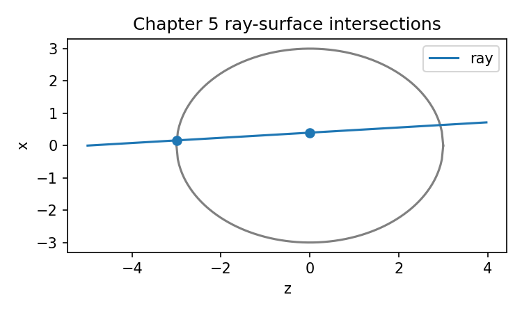
Chapter 5: How a Ray Hits a Curved Surface
A lens drawing makes this step look effortless.
A ray travels forward. It reaches a glass surface. It bends. Then it continues.
In the drawing, the contact point is obvious because your eye sees the line touch the curve. But a program does not see that picture. A program has only numbers:
ray position
ray direction
surface position
surface shape
From those numbers, it must answer a very specific question:
At what point does this ray hit this surface?
This is ray-surface intersection.
It is one of the most important calculations in geometric ray tracing, and it is also one of the easiest to skip in an explanation. Many books and manuals show rays bending at surfaces, then move quickly to Snell’s law. But Snell’s law cannot act until we know where the ray meets the surface and what the surface normal is at that point.
So this chapter slows down.
We will not refract yet. That is Chapter 6. Here, we do only the geometry:
ray + plane  → intersection point
ray + sphere → intersection point
intersection point → aperture check
intersection point → surface normal
By the end of this chapter, a ray will be able to collide with a plane or spherical surface. It will not yet bend. But it will know exactly where bending should happen.
That is a large step.
The problem in one line
From Chapter 4, our ray is:
r(t) = r0 + t d
where:
r0 = ray starting position
d  = normalized ray direction
t  = forward distance parameter
A surface is a set of points satisfying some equation.
For a plane perpendicular to the optical axis:
z = z_v
For a sphere:
(x - cx)² + (y - cy)² + (z - cz)² = R²
Intersection means:
Find the value of
tsuch that the ray pointr(t)lies on the surface.
That is the whole idea.
For a plane, the equation is linear.
For a sphere, the equation becomes quadratic.
For more complex aspheric or freeform surfaces, the equation may need numerical solving. But planes and spheres are enough to build the foundation.
A surface has a vertex
Before writing intersection code, we need one more piece of optical vocabulary.
In a sequential lens prescription, each surface has a vertex position along the optical axis. If the first physical surface is at z = 0, and its thickness is 5 mm, then the next surface vertex is at z = 5 mm.
The vertex is the point where the surface crosses the optical axis.
For a rotationally symmetric spherical surface, we can think of the surface as being placed at a vertex position z_v, with a signed radius R.
Using the convention from earlier chapters:
light generally travels in +z
surface vertex is at z = z_v
signed radius R gives the center of curvature at z = z_v + R
So if:
z_v = 0
R = +50 mm
the sphere center lies at:
z_c = 50 mm
If:
z_v = 5
R = -50 mm
the sphere center lies at:
z_c = -45 mm
This signed-radius convention lets one formula describe both convex and concave surfaces in a sequential optical system.
We will use this model for teaching code.
A small surface class for intersection
The Surface class from earlier chapters stored radius, thickness, material, semi-diameter, and surface type. For intersection, we also need the actual vertex position z.
In a full lens system, we can compute vertex positions from the thickness column. For this chapter, it is helpful to use a separate small class that stores the vertex directly.
from dataclasses import dataclass
from typing import Optional
import math
import numpy as np

@dataclass
class IntersectableSurface:
    radius: float
    z_vertex: float
    semi_diameter: Optional[float] = None
    surface_type: str = "spherical"
    comment: str = ""
This is not meant to replace the prescription data structure permanently. It is a teaching object. It lets us focus on intersection without carrying the whole lens system around.
For example:
front_surface = IntersectableSurface(
    radius=50.0,
    z_vertex=0.0,
    semi_diameter=10.0,
    comment="front spherical surface"
)

image_plane = IntersectableSurface(
    radius=float("inf"),
    z_vertex=50.0,
    semi_diameter=None,
    surface_type="plane",
    comment="image plane"
)
The front surface is spherical. The image plane is a plane at z = 50.
Now we can ask rays to hit them.
Ray-plane intersection
Start with the easiest case.
A plane perpendicular to the optical axis has equation:
z = z_v
The ray is:
r(t) = r0 + t d
If we write only the z coordinate:
z(t) = z0 + t dz
Set it equal to the plane:
z_v = z0 + t dz
Solve for t:
t = (z_v - z0) / dz
This is the same calculation we used in Chapter 4 to propagate to a z plane. Now we will treat it formally as a surface intersection.
def intersect_plane_z(ray, z_plane, eps=1e-12):
    """Return forward distance t where ray intersects plane z = z_plane.

    Returns None if the ray is parallel to the plane or the intersection
    is not in the forward direction.
    """
    dz = ray.direction[2]

    if abs(dz) < eps:
        return None

    t = (z_plane - ray.position[2]) / dz

    if t <= eps:
        return None

    return t
The eps value avoids treating tiny numerical noise as a real forward intersection. In ray tracing, this matters. After a ray has just landed on a surface, we do not want the next intersection test to rediscover the same surface at t = 0.
Test it:
ray = Ray(position=[0, 0, 0], direction=[0.1, 0, 1.0])

t = intersect_plane_z(ray, z_plane=50.0)
p = ray.point_at(t)

print("t =", t)
print("point =", p)
The output should show a point with z = 50. The x value will be nonzero because the ray is tilted.
That is already an intersection.
No drawing was needed.
Turning intersection into an event
We can write a helper that moves the ray to the plane.
def propagate_to_plane(ray, z_plane, refractive_index=1.0):
    t = intersect_plane_z(ray, z_plane)

    if t is None:
        ray.stop(f"missed plane z={z_plane}")
        return ray

    ray.propagate(t, refractive_index=refractive_index)
    return ray
This uses the Ray class from Chapter 4. It updates both position and optical path length.
ray = Ray(position=[0, 0, 0], direction=[0.1, 0, 1.0])
propagate_to_plane(ray, z_plane=50.0)

print(ray.position)
print(ray.opl)
print(ray.alive)
The ray is now sitting on the plane. If this were an image plane, we could record its x and y coordinates as a spot diagram point.
For a plane surface, intersection is easy. The real fun begins with spheres.
Ray-sphere intersection
A spherical optical surface is part of a sphere.
Let its center be:
C = [0, 0, z_c]
and its radius magnitude be:
|R|
A point p = [x, y, z] lies on the sphere if:
||p - C||² = R²
The ray point is:
p(t) = r0 + t d
Substitute the ray into the sphere equation:
||r0 + t d - C||² = R²
This becomes a quadratic equation in t.
Let:
oc = r0 - C
Then:
||oc + t d||² = R²
Expand:
(d · d)t² + 2(d · oc)t + (oc · oc - R²) = 0
So:
a = d · d
b = 2(d · oc)
c = oc · oc - R²
Solve:
t = (-b ± sqrt(b² - 4ac)) / (2a)
Because our ray direction is normalized, a should be 1. But we will compute it anyway. That makes the function more robust.
The discriminant tells us whether the ray hits the sphere:
discriminant = b² - 4ac
If the discriminant is negative, there is no real intersection.
If it is zero, the ray is tangent to the sphere.
If it is positive, the ray intersects the sphere at two mathematical points.
For optical ray tracing, we usually want the nearest positive intersection.
Here is the code:
def sphere_center_from_surface(surface):
    """Return the center of curvature for a spherical surface."""
    if math.isinf(surface.radius):
        return None

    return np.array([0.0, 0.0, surface.z_vertex + surface.radius], dtype=float)

def intersect_sphere(ray, surface, eps=1e-9):
    """Return forward distance t where ray intersects a spherical surface.

    The surface is represented by a vertex position z_vertex and signed radius.
    The sphere center is at z_vertex + radius.
    """
    if math.isinf(surface.radius):
        return intersect_plane_z(ray, surface.z_vertex, eps=eps)

    center = sphere_center_from_surface(surface)
    radius_abs = abs(surface.radius)

    oc = ray.position - center

    a = float(np.dot(ray.direction, ray.direction))
    b = 2.0 * float(np.dot(ray.direction, oc))
    c = float(np.dot(oc, oc) - radius_abs * radius_abs)

    disc = b * b - 4.0 * a * c

    if disc < 0:
        return None

    sqrt_disc = math.sqrt(max(disc, 0.0))

    t1 = (-b - sqrt_disc) / (2.0 * a)
    t2 = (-b + sqrt_disc) / (2.0 * a)

    candidates = [t for t in (t1, t2) if t > eps]

    if not candidates:
        return None

    return min(candidates)
Now test an on-axis ray hitting the first surface of a spherical lens.
surface = IntersectableSurface(
    radius=50.0,
    z_vertex=0.0,
    semi_diameter=10.0,
    comment="front surface"
)

ray = Ray(position=[0.0, 0.0, -20.0], direction=[0.0, 0.0, 1.0])

t = intersect_sphere(ray, surface)
p = ray.point_at(t)

print("t =", t)
print("intersection =", p)
For an on-axis ray, the intersection should be at the vertex:
[0, 0, 0]
or very close to it.
Now try an off-axis parallel ray:
ray = Ray(position=[5.0, 0.0, -20.0], direction=[0.0, 0.0, 1.0])

t = intersect_sphere(ray, surface)
p = ray.point_at(t)

print("t =", t)
print("intersection =", p)
The x coordinate should remain 5, while z should be slightly positive. Why positive? Because a spherical surface with center at z = 50 bulges toward the incoming ray. At height x = 5, the surface point lies slightly to the right of the vertex along z.
This is the sag of the surface appearing naturally from intersection geometry.
Comparing intersection with sag
From Chapter 2, the sag of a spherical surface can be computed as:
sag(r) = R - sign(R) sqrt(R² - r²)
There are several equivalent forms depending on sign convention. For our vertex-and-center convention, the spherical surface satisfies:
x² + y² + (z - (z_v + R))² = R²
Solving for the branch that passes through the vertex gives:
z = z_v + R - sign(R) sqrt(R² - r²)
where:
r² = x² + y²
Let us implement it:
def spherical_sag(x, y, surface):
    """Return z coordinate of a spherical surface at transverse point (x, y)."""
    if math.isinf(surface.radius):
        return surface.z_vertex

    R = surface.radius
    r2 = x*x + y*y
    R2 = R*R

    if r2 > R2:
        return None

    return surface.z_vertex + R - math.copysign(math.sqrt(R2 - r2), R)
Now compare the off-axis intersection:
x, y, z = p
print("intersection z:", z)
print("sag z:", spherical_sag(x, y, surface))
They should match.
This is a good sanity check. The ray-sphere intersection and the surface sag describe the same geometry from two different directions:
intersection: where does this ray meet the surface?
sag: where is the surface at this x, y?
Both are useful.
Why there are two sphere intersections
A line can pass through a sphere in two places.
For a full sphere, this is obvious. The ray enters the sphere on the near side and exits on the far side.
But an optical surface is not the whole sphere. It is a local patch near the vertex. In sequential ray tracing, we normally want the first forward intersection with that surface.
That is why intersect_sphere chooses the smallest positive t.
This works for many teaching examples, but there is a subtle point.
In a real sequential optical system, the expected surface is the next surface in the prescription. The ray may mathematically intersect the far side of the sphere too, but that is not the physical surface patch we mean. Aperture checks and sequential geometry help reject irrelevant intersections.
For ordinary spherical lens surfaces near the optical axis, choosing the nearest positive intersection is the right first rule.
When systems become more complex, robust ray tracing needs additional safeguards:
surface aperture limits
expected propagation direction
local coordinate systems
avoidance of self-intersection
handling of coordinate breaks
surface branch selection
We do not need all of that yet. But it is good to know that professional ray tracers are careful here for a reason.
Aperture check
Finding a mathematical intersection is not enough.
The ray might hit the infinite sphere outside the clear optical area.
A lens surface has a semi-diameter. If the intersection point is too far from the optical axis, the ray is blocked.
For a circular clear aperture:
x² + y² <= semi_diameter²
In code:
def inside_surface_aperture(point, surface):
    """Return True if point is inside the circular clear aperture."""
    if surface.semi_diameter is None:
        return True

    x, y, _ = point
    return x*x + y*y <= surface.semi_diameter * surface.semi_diameter
Test:
surface = IntersectableSurface(
    radius=50.0,
    z_vertex=0.0,
    semi_diameter=10.0
)

points = [
    np.array([0.0, 0.0, 0.0]),
    np.array([5.0, 0.0, 0.0]),
    np.array([10.0, 0.0, 0.0]),
    np.array([11.0, 0.0, 0.0]),
]

for p in points:
    print(p, inside_surface_aperture(p, surface))
The point at x = 11 is outside.
This check may feel mundane. It is not. Aperture clipping affects ray bundles, vignetting, spot diagrams, pupil sampling, illumination, and later image quality calculations.
A ray that hits the mathematical sphere but outside the clear aperture should not continue as though it passed through the lens.
A complete hit record
It is useful to return more than just t.
When a ray hits a surface, we may want:
distance t
intersection point
whether it is inside the aperture
surface normal
surface reference
Let us define a small hit record.
@dataclass
class SurfaceHit:
    t: float
    point: np.ndarray
    normal: np.ndarray
    inside_aperture: bool
    surface: IntersectableSurface
Now we need the normal.
Surface normal for a plane
For a plane z = z_v, a normal can be:
[0, 0, 1]
or:
[0, 0, -1]
Both are geometrically valid. The sign matters for refraction, because Snell’s law uses the normal direction.
For this chapter, we will define a default geometric normal for a plane as:
[0, 0, 1]
Then in Chapter 6, we will orient the normal relative to the incoming ray before applying the vector refraction formula.
def plane_normal():
    return np.array([0.0, 0.0, 1.0])
Surface normal for a sphere
For a sphere, the normal at a point points along the radius from the center to the point.
normal = normalize(point - center)
In code:
def surface_normal(point, surface):
    """Return a geometric unit normal at a point on the surface."""
    if math.isinf(surface.radius) or surface.surface_type == "plane":
        return plane_normal()

    center = sphere_center_from_surface(surface)
    return normalize(point - center)
Test on the vertex of a positive-radius front surface:
surface = IntersectableSurface(radius=50.0, z_vertex=0.0)
point = np.array([0.0, 0.0, 0.0])

print(surface_normal(point, surface))
The normal is:
[0, 0, -1]
Why negative z? Because the sphere center is at z = +50, and the vertex point is at z = 0. The vector from center to vertex points toward negative z.
For the back surface of the same biconvex lens:
back_surface = IntersectableSurface(radius=-50.0, z_vertex=5.0)
point = np.array([0.0, 0.0, 5.0])

print(surface_normal(point, back_surface))
The normal is:
[0, 0, 1]
This is good. The two spherical surfaces have opposite geometric normals at their vertices.
Do not worry yet about whether the normal points “the right way” for refraction. In Chapter 6, we will handle orientation carefully.
For now, the normal is a property of the surface geometry.
The full intersection function
Now combine the pieces.
def intersect_surface(ray, surface, eps=1e-9):
    """Return a SurfaceHit if ray intersects the surface, otherwise None."""
    if surface.surface_type == "plane" or math.isinf(surface.radius):
        t = intersect_plane_z(ray, surface.z_vertex, eps=eps)
    else:
        t = intersect_sphere(ray, surface, eps=eps)

    if t is None:
        return None

    point = ray.point_at(t)
    normal = surface_normal(point, surface)
    inside = inside_surface_aperture(point, surface)

    return SurfaceHit(
        t=t,
        point=point,
        normal=normal,
        inside_aperture=inside,
        surface=surface,
    )
Test it:
surface = IntersectableSurface(
    radius=50.0,
    z_vertex=0.0,
    semi_diameter=10.0,
    comment="front surface"
)

ray = Ray(position=[5.0, 0.0, -20.0], direction=[0.0, 0.0, 1.0])

hit = intersect_surface(ray, surface)

print("t:", hit.t)
print("point:", hit.point)
print("normal:", hit.normal)
print("inside aperture:", hit.inside_aperture)
This is the first time our code has answered the full geometric question.
The ray hit the surface. We know where. We know the normal. We know whether the point is inside the clear aperture.
The next chapter will use the normal and the refractive indices to compute the outgoing ray direction.
Moving the ray to the hit point
A hit record tells us where the ray would hit. But the ray object itself has not moved yet.
We can write:
def propagate_to_surface(ray, surface, refractive_index=1.0):
    """Move a ray to a surface intersection if possible.

    Does not refract. It only propagates to the hit point and checks aperture.
    """
    hit = intersect_surface(ray, surface)

    if hit is None:
        ray.stop(f"missed surface: {surface.comment}")
        return None

    if not hit.inside_aperture:
        ray.propagate(hit.t, refractive_index=refractive_index)
        ray.stop(f"blocked by aperture: {surface.comment}")
        return hit

    ray.propagate(hit.t, refractive_index=refractive_index)

    ray.history.append({
        "event": "surface_hit",
        "surface": surface.comment,
        "point": hit.point.copy(),
        "normal": hit.normal.copy(),
        "inside_aperture": hit.inside_aperture,
    })

    return hit
Try it:
ray = Ray(position=[5.0, 0.0, -20.0], direction=[0.0, 0.0, 1.0])

hit = propagate_to_surface(ray, surface)

print("ray position:", ray.position)
print("ray alive:", ray.alive)
print("stop reason:", ray.stop_reason)
The ray should now sit on the spherical surface.
Again, it has not bent. That restraint is intentional. We want each step to be inspectable.
Chapter 5: where does the ray hit?
Chapter 6: where does it go after hitting?
Do not mix those too early.
Visualizing ray-sphere hits
A picture helps, as long as we remember that the picture is derived from the computation.
Let us trace several parallel rays into a spherical surface and plot their hit points.
import matplotlib.pyplot as plt

surface = IntersectableSurface(
    radius=50.0,
    z_vertex=0.0,
    semi_diameter=10.0,
    comment="front spherical surface"
)

rays = [
    Ray(position=[x, 0.0, -20.0], direction=[0.0, 0.0, 1.0])
    for x in np.linspace(-9.0, 9.0, 7)
]

hit_points = []

for ray in rays:
    hit = intersect_surface(ray, surface)
    if hit is not None and hit.inside_aperture:
        hit_points.append(hit.point)

hit_points = np.array(hit_points)

# Draw surface profile in x-z plane.
xs = np.linspace(-10.0, 10.0, 300)
zs = [spherical_sag(x, 0.0, surface) for x in xs]

plt.plot(zs, xs, label="spherical surface")

# Draw incoming ray segments and hit points.
for ray, hp in zip(rays, hit_points):
    plt.plot([ray.position[2], hp[2]], [ray.position[0], hp[0]], linewidth=0.8)

plt.scatter(hit_points[:, 2], hit_points[:, 0], label="hit points")
plt.xlabel("z [mm]")
plt.ylabel("x [mm]")
plt.title("Parallel rays hitting a spherical surface")
plt.gca().set_aspect("equal", adjustable="box")
plt.legend()
plt.show()
This plot should show straight parallel rays reaching different points on the curved surface. The off-axis rays hit the surface at different z positions because the surface is curved.
This is not merely a drawing. Every contact point was computed.
That distinction is the point of the chapter.
What if the ray misses?
A ray may miss a sphere.
For example, if the ray travels far outside the surface:
ray = Ray(position=[100.0, 0.0, -20.0], direction=[0.0, 0.0, 1.0])
hit = intersect_surface(ray, surface)

print(hit)
This may return None, or it may mathematically hit the large parent sphere depending on geometry. But it should fail the aperture check if the surface semi-diameter is small.
That is why both checks matter:
Does the ray intersect the mathematical surface?
Is the intersection inside the clear aperture?
For optical surfaces, the second question is often just as important as the first.
A ray can hit the sphere but miss the lens.
Tangent rays and numerical precision
If a ray just grazes a sphere, the quadratic discriminant is close to zero. Numerically, this can be delicate.
In exact math:
discriminant = 0
means tangent.
In floating-point computation, a value that should be zero might appear as:
-1e-14
because of rounding.
That is why some ray tracers use tolerances. A robust function may treat very small negative discriminants as zero.
We used:
sqrt_disc = math.sqrt(max(disc, 0.0))
but only after checking:
if disc < 0:
    return None
For teaching code, this is acceptable. For more robust code, we might write:
if disc < -eps:
    return None
disc = max(disc, 0.0)
This would allow tiny negative values caused by numerical roundoff.
Here is a more tolerant version:
def intersect_sphere_tolerant(ray, surface, eps=1e-9):
    if math.isinf(surface.radius):
        return intersect_plane_z(ray, surface.z_vertex, eps=eps)

    center = sphere_center_from_surface(surface)
    radius_abs = abs(surface.radius)
    oc = ray.position - center

    a = float(np.dot(ray.direction, ray.direction))
    b = 2.0 * float(np.dot(ray.direction, oc))
    c = float(np.dot(oc, oc) - radius_abs * radius_abs)

    disc = b*b - 4.0*a*c

    if disc < -eps:
        return None

    disc = max(disc, 0.0)
    sqrt_disc = math.sqrt(disc)

    t1 = (-b - sqrt_disc) / (2.0*a)
    t2 = (-b + sqrt_disc) / (2.0*a)

    candidates = [t for t in (t1, t2) if t > eps]

    if not candidates:
        return None

    return min(candidates)
Numerical tolerance is not an advanced luxury. It is part of making geometry work on finite-precision machines.
Intersections and local coordinates
So far, all surfaces are centered on the z axis. That is enough for early chapters.
A real optical design program needs local coordinates. A surface may be tilted, decentered, or placed after a coordinate break. The ray may need to be transformed into the surface’s local coordinate system, intersected there, and transformed back.
The general pattern is:
global ray
→ transform into local surface coordinates
→ compute intersection
→ compute local normal
→ transform point and normal back to global coordinates
This sounds like a complication, and it is. But notice that the basic intersection problem remains the same. The local coordinate system is there to make the surface equation simpler.
We will not implement coordinate breaks in this book’s core teaching code. That would distract from the main computation chain. But when you see a professional library handling tilted mirrors, prisms, off-axis systems, or freeform surfaces, remember that it is doing this kind of coordinate bookkeeping.
The skeleton is still:
ray + surface equation → t → point → normal
The coordinate transforms just prepare the inputs and return the result to the global system.
Building surface vertices from a prescription
In Chapter 2, a lens prescription gave us thicknesses. For intersection, we need surface vertex positions.
Let us write a helper that converts a sequence of prescription surfaces into intersectable surfaces with z positions.
Assume we have a Surface class like before:
@dataclass
class Surface:
    radius: float
    thickness: float
    material_after: str = "air"
    semi_diameter: Optional[float] = None
    conic: float = 0.0
    is_stop: bool = False
    surface_type: str = "spherical"
    comment: str = ""
Now convert:
def build_intersectable_surfaces(prescription_surfaces):
    """Convert prescription surfaces into surfaces with vertex z positions.

    Skips an object-at-infinity row if present.
    """
    surfaces = prescription_surfaces

    if surfaces and math.isinf(surfaces[0].thickness):
        surfaces = surfaces[1:]

    z = 0.0
    result = []

    for s in surfaces:
        surface_type = s.surface_type

        if math.isinf(s.radius):
            surface_type = "plane"

        result.append(IntersectableSurface(
            radius=s.radius,
            z_vertex=z,
            semi_diameter=s.semi_diameter,
            surface_type=surface_type,
            comment=s.comment,
        ))

        if not math.isinf(s.thickness):
            z += s.thickness

    return result
Now a lens prescription can feed intersection code.
This is the first time the data structure from Chapter 2 starts to move real rays from Chapter 4.
The chain is becoming executable:
prescription thicknesses
→ surface vertex positions
→ ray-surface intersections
→ hit points and normals
A no-refraction trace through two surfaces
Let us trace a ray to the two surfaces of a singlet, but without bending it.
This is physically wrong as optics, but useful as geometry.
prescription = [
    Surface(
        radius=float("inf"),
        thickness=float("inf"),
        surface_type="object",
        comment="object at infinity"
    ),
    Surface(
        radius=50.0,
        thickness=5.0,
        material_after="N-BK7",
        semi_diameter=10.0,
        comment="front surface"
    ),
    Surface(
        radius=-50.0,
        thickness=45.0,
        material_after="air",
        semi_diameter=10.0,
        comment="back surface"
    ),
    Surface(
        radius=float("inf"),
        thickness=0.0,
        surface_type="image",
        comment="image plane"
    ),
]

surfaces = build_intersectable_surfaces(prescription)

ray = Ray(position=[3.0, 0.0, -20.0], direction=[0.0, 0.0, 1.0])

for s in surfaces:
    hit = propagate_to_surface(ray, s, refractive_index=1.0)

    if hit is None or not ray.alive:
        break

    print(s.comment, ray.position, "normal", hit.normal)
The ray passes through the front surface, then the back surface, then reaches the image plane. It does not bend, so it is not a real optical trace. But it confirms that the geometry is working.
This kind of intermediate test is extremely useful.
Before adding refraction, make sure intersections work.
Before adding wavefronts, make sure refraction works.
Before adding PSF, make sure OPD works.
A black box is often just too many untested steps stacked together.
The image plane is just another plane intersection
The image plane is often special in interpretation, but geometrically it is simple.
It is usually represented as a plane perpendicular to the optical axis:
z = z_image
When rays reach it, we record their transverse coordinates:
x_image, y_image
Those coordinates become spot diagram points.
The image plane does not need refraction if it is only an evaluation surface. It is where we measure the ray, not necessarily a physical boundary.
That is why our build_intersectable_surfaces function can treat an infinite-radius image surface as a plane.
Later, in a full trace, the image plane will be the last surface. Rays that reach it contribute to geometric image analysis.
Surface normal and refraction are separate jobs
It is tempting to jump straight from intersection to bending. Let us resist that for one more section.
At a surface hit, we now know:
point
normal
material before
material after
ray direction
wavelength
The refraction calculation will use:
incoming direction
surface normal
n_before
n_after
But the normal itself is a geometric object. It should be computed before and independently from Snell’s law.
This separation keeps the code clean:
intersection code:
    returns point and normal

material code:
    returns n_before and n_after

refraction code:
    returns new direction
If all of that is mixed into one function, debugging becomes painful.
When a ray bends incorrectly, you will not know whether the point was wrong, the normal was wrong, the refractive index was wrong, or the vector formula was wrong.
Small functions are not just stylistic preference. They make optical errors visible.
A preview of the next step
At the end of this chapter, a ray hitting a spherical surface has an incoming direction and a normal.
For example:
ray = Ray(position=[5.0, 0.0, -20.0], direction=[0.0, 0.0, 1.0])
surface = IntersectableSurface(radius=50.0, z_vertex=0.0, semi_diameter=10.0)

hit = intersect_surface(ray, surface)

print("incoming direction:", ray.direction)
print("surface normal:", hit.normal)
The incoming direction might be:
[0, 0, 1]
The normal will be tilted because the ray hit the curved surface away from the axis:
normal ≈ [small x component, 0, mostly negative z]
That tilted normal is exactly why an off-axis ray bends differently from an on-axis ray. Snell’s law does not see the whole lens drawing. It sees the local surface normal at the hit point.
This is the local nature of refraction.
A curved lens is not magic. It is many local surface normals changing from point to point.
That is a beautiful thought, and also a computationally useful one.
Common mistakes in ray-surface intersection
Let us name the traps before they bite.
Mistake 1: Forgetting to choose the forward intersection
The quadratic equation gives mathematical roots. Some may lie behind the ray. Use positive t values and choose the nearest valid one.
Mistake 2: Ignoring aperture limits
A ray can intersect the parent sphere but outside the actual lens surface. Always check the clear aperture.
Mistake 3: Confusing radius sign with radius magnitude
The signed radius locates the center of curvature. The sphere equation uses the magnitude of the radius.
center z = z_vertex + R
sphere radius = |R|
Mistake 4: Using the wrong surface branch
A full sphere has two sides. A sequential optical surface is a local patch near its vertex. In ordinary cases, the nearest positive intersection works, but more complex systems require care.
Mistake 5: Not using tolerances
Floating-point calculations are not exact. Very small negative discriminants or tiny t values can cause false misses or self-intersections.
Mistake 6: Mixing sag and intersection logic
Sag gives surface height for a known transverse coordinate. Intersection solves where a ray meets the surface. They are related, but they answer different questions.
Mistake 7: Computing refraction before verifying the hit
Do not refract a ray that missed the surface or was blocked by the aperture.
Mistake 8: Losing the normal direction
The surface normal must be normalized and stored carefully. The refraction chapter will need it.
What this chapter gives us
We now have the geometric core of ray tracing.
We can:
represent a plane surface
represent a spherical surface with signed radius
compute ray-plane intersection
compute ray-sphere intersection
choose the nearest forward hit
check whether the hit is inside the clear aperture
compute the surface normal at the hit point
move the ray to the surface
record the hit
This is not a small accomplishment.
A ray in Chapter 4 could only travel through empty space.
A ray after Chapter 5 can find the glass.
It still cannot bend. But that is now the only missing action for a basic real ray trace.
The next chapter will add it.
We will take the incoming direction, the surface normal, and the refractive indices from Chapter 3. Then we will compute the outgoing direction using Snell’s law in vector form.
That is the moment the ray will finally do what the drawing has always shown:
it will hit the surface
and change direction
But this time, we will know exactly where that happened, which normal was used, which indices were used, and how the new direction was calculated.
That is how a software command becomes a calculation you can inspect.
Generated validation figure