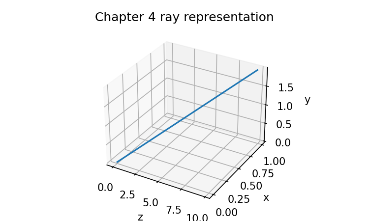
Chapter 4: How to Represent a Ray

A ray in an optical drawing looks effortless.

It is just a line.

It leaves the object, passes through the lens, bends at the surfaces, and lands near the image plane. If several rays are drawn together, they form a neat fan. If they are traced through a good lens, they gather. If the lens is poor, they spread. The picture is intuitive enough that we may forget a simple fact:

A drawn ray is not yet a computational ray.

A program cannot trace a sketch. It needs numbers.

It needs to know where the ray starts, which direction it travels, what wavelength it carries, whether it is still valid, and eventually how much optical path length it has accumulated. If we want to build spot diagrams, wavefront maps, PSF, and MTF from first principles, we must first make this object explicit.

This chapter is about that object.

Not the surface yet. Not refraction yet. Not the image quality yet.

Just the ray.

That may feel like a small topic, but it is the root of everything that follows. A ray tracer is not a magic optical engine. It is a loop that repeatedly performs a few operations on a ray:

start with a ray
→ find where it hits the next surface
→ compute the surface normal
→ refract or reflect the ray
→ propagate to the next surface
→ repeat

If the ray itself is vague, the loop becomes vague.

So let us make the ray concrete.

A ray is a parametric line with optical baggage

The basic geometric form of a ray is:

r(t) = r0 + t d

Here:

r0 = starting point of the ray
d  = direction vector
t  = distance-like parameter along the ray

If d is normalized so that its length is 1, then t has the same length unit as the coordinates. If positions are in millimeters, then t is in millimeters.

This is a very useful convention.

For example, if:

r0 = [0, 0, 0]
d  = [0, 0, 1]

then:

r(10) = [0, 0, 10]

The ray has moved 10 mm in the positive z direction.

If the ray is tilted:

d = [0.1, 0, 0.995]

then moving forward changes both x and z.

This is the geometry. But an optical ray needs more than geometry. It should also carry at least:

wavelength
intensity
optical path length
valid / invalid status

Later, a more advanced ray may also carry polarization state, phase, surface history, or differential information for optimization. We do not need all of that yet.

For now, our ray will know five things:

position
direction
wavelength
intensity
optical path length

and one status flag:

alive or stopped

That is enough to begin.

Normalize the direction, always

The direction vector should be normalized.

That means:

||d|| = 1

or:

sqrt(dx² + dy² + dz²) = 1

Why insist on this?

Because it makes propagation clean. If d has unit length, then t is physical distance. Moving the ray by t = 5.0 means moving it 5.0 mm through space.

If d is not normalized, then t becomes harder to interpret. A ray with direction [0, 0, 10] and a ray with direction [0, 0, 1] point the same way, but r0 + t d moves them by very different amounts for the same t.

That is not what we want.

So the ray constructor should normalize the direction immediately.

import numpy as np

def normalize(v):
    """Return a unit-length copy of vector v."""
    v = np.asarray(v, dtype=float)
    norm = np.linalg.norm(v)

    if norm == 0:
        raise ValueError("Cannot normalize a zero vector.")

    return v / norm

Test it:

d = normalize([0, 0, 10])
print(d)
print(np.linalg.norm(d))

The result is:

[0. 0. 1.]
1.0

This tiny helper function will appear everywhere. It is one of the quiet tools that keeps ray tracing stable.

A first Ray class

Let us write a minimal Ray class.

from dataclasses import dataclass, field
import numpy as np

@dataclass
class Ray:
    position: np.ndarray
    direction: np.ndarray
    wavelength_um: float = 0.5876
    intensity: float = 1.0
    opl: float = 0.0
    alive: bool = True
    stop_reason: str = ""
    history: list = field(default_factory=list)

    def __post_init__(self):
        self.position = np.asarray(self.position, dtype=float)
        self.direction = normalize(self.direction)

        if self.position.shape != (3,):
            raise ValueError("Ray position must be a 3D vector.")

        if self.direction.shape != (3,):
            raise ValueError("Ray direction must be a 3D vector.")

        if self.wavelength_um <= 0:
            raise ValueError("Wavelength must be positive.")

        if self.intensity < 0:
            raise ValueError("Intensity cannot be negative.")

    def point_at(self, t):
        """Return the point r(t) = r0 + t d."""
        return self.position + t * self.direction

    def copy(self):
        """Return a copy of the ray."""
        return Ray(
            position=self.position.copy(),
            direction=self.direction.copy(),
            wavelength_um=self.wavelength_um,
            intensity=self.intensity,
            opl=self.opl,
            alive=self.alive,
            stop_reason=self.stop_reason,
            history=list(self.history),
        )

This is not yet a ray tracer. It is a well-defined object that a ray tracer can use.

A ray has a position and a direction. It knows its wavelength. It has an intensity. It has an accumulated optical path length, opl. It can be alive or stopped. It can store history if we want to inspect where it has been.

Now create a ray:

ray = Ray(
    position=[0.0, 0.0, 0.0],
    direction=[0.1, 0.0, 1.0],
    wavelength_um=0.5876,
)

print("position:", ray.position)
print("direction:", ray.direction)
print("direction length:", np.linalg.norm(ray.direction))
print("point at t=10:", ray.point_at(10.0))

The direction is automatically normalized. The point at t = 10 lies 10 mm along that normalized direction.

This is the first real computational ray.

The direction vector is not the same as an angle

In simple two-dimensional drawings, we often describe rays by an angle.

For example:

a ray tilted by 5 degrees from the optical axis

That is fine for human discussion. But in three-dimensional computation, a direction vector is often more convenient.

A direction vector can represent tilt in both x and y. It also works naturally with dot products, surface normals, vector refraction, and intersections.

Still, it is useful to create a direction from angles.

Let the optical axis be the positive z axis. A ray tilted in the x-z plane by angle θx has direction:

d = [sin θx, 0, cos θx]

For small field angles, this is enough.

import math

def direction_from_x_angle(theta_x_deg):
    """Create a unit direction vector tilted in the x-z plane."""
    theta = math.radians(theta_x_deg)
    return np.array([math.sin(theta), 0.0, math.cos(theta)])

for angle in [0.0, 5.0, 10.0]:
    print(angle, direction_from_x_angle(angle))

For tilts in both x and y, we can write a simple helper. One clean construction is to point the ray toward a plane at z = 1:

def direction_from_field_angles(theta_x_deg=0.0, theta_y_deg=0.0):
    """Create a direction vector from approximate field angles.

    The ray points toward (tan θx, tan θy, 1).
    This is convenient for field-angle based examples.
    """
    tx = math.tan(math.radians(theta_x_deg))
    ty = math.tan(math.radians(theta_y_deg))
    return normalize([tx, ty, 1.0])

Test it:

print(direction_from_field_angles(0.0, 0.0))
print(direction_from_field_angles(5.0, 0.0))
print(direction_from_field_angles(0.0, 5.0))
print(direction_from_field_angles(5.0, 5.0))

This helper is not a full field model. It is just a practical way to generate rays that travel roughly along the optical axis with a specified angular tilt.

Later, when we generate bundles of rays from field points and pupil coordinates, this kind of function will become part of a larger sampling routine.

Propagating a ray by distance

The simplest operation on a ray is propagation through a uniform medium.

If the ray moves a physical distance s, its new position is:

r_new = r_old + s d

If the medium has refractive index n, the optical path length increases by:

ΔOPL = n s

This deserves attention.

Geometric distance and optical path length are not the same thing. A ray traveling 10 mm through air has optical path length about 10 mm if n ≈ 1. The same geometric distance through glass with n = 1.5 has optical path length about 15 mm.

This will matter later when we compute OPD. Wavefront error is not built from plain geometric distance alone. It depends on optical path.

Let us implement propagation.

@dataclass
class Ray:
    position: np.ndarray
    direction: np.ndarray
    wavelength_um: float = 0.5876
    intensity: float = 1.0
    opl: float = 0.0
    alive: bool = True
    stop_reason: str = ""
    history: list = field(default_factory=list)

    def __post_init__(self):
        self.position = np.asarray(self.position, dtype=float)
        self.direction = normalize(self.direction)

        if self.position.shape != (3,):
            raise ValueError("Ray position must be a 3D vector.")
        if self.direction.shape != (3,):
            raise ValueError("Ray direction must be a 3D vector.")
        if self.wavelength_um <= 0:
            raise ValueError("Wavelength must be positive.")
        if self.intensity < 0:
            raise ValueError("Intensity cannot be negative.")

    def point_at(self, t):
        return self.position + t * self.direction

    def propagate(self, distance, refractive_index=1.0):
        """Move the ray forward by geometric distance.

        distance is in the same length unit as position, usually mm.
        refractive_index is dimensionless.
        """
        if not self.alive:
            return self

        if distance < 0:
            raise ValueError("Propagation distance should be non-negative.")

        old_position = self.position.copy()
        self.position = self.point_at(distance)
        self.opl += refractive_index * distance

        self.history.append({
            "event": "propagate",
            "from": old_position,
            "to": self.position.copy(),
            "distance": distance,
            "n": refractive_index,
            "opl": self.opl,
        })

        return self

    def stop(self, reason):
        self.alive = False
        self.stop_reason = reason
        self.history.append({
            "event": "stop",
            "reason": reason,
            "position": self.position.copy(),
        })
        return self

    def copy(self):
        return Ray(
            position=self.position.copy(),
            direction=self.direction.copy(),
            wavelength_um=self.wavelength_um,
            intensity=self.intensity,
            opl=self.opl,
            alive=self.alive,
            stop_reason=self.stop_reason,
            history=list(self.history),
        )

Now try it:

ray = Ray([0, 0, 0], [0, 0, 1], wavelength_um=0.5876)
ray.propagate(10.0, refractive_index=1.0)

print(ray.position)
print(ray.opl)

The output is:

[ 0.  0. 10.]
10.0

Through glass:

ray = Ray([0, 0, 0], [0, 0, 1], wavelength_um=0.5876)
ray.propagate(10.0, refractive_index=1.5)

print(ray.position)
print(ray.opl)

The position is still [0, 0, 10], but the optical path length is 15.0.

That small distinction is one of the bridges from geometric ray tracing to wavefront computation.

Propagating to a z plane

In sequential optical systems, many useful surfaces are arranged along the z axis. Even before we handle curved surfaces, it is useful to ask:

Where does this ray meet the plane z = z_target?

For a ray:

r(t) = r0 + t d

the z coordinate is:

z(t) = z0 + t dz

Set this equal to z_target:

z_target = z0 + t dz

Solve for t:

t = (z_target - z0) / dz

This formula is simple, but it already teaches an important habit: intersection is usually parameter solving. We find the parameter t that places the ray on the target surface.

Here is the code:

def distance_to_z_plane(ray, z_target, eps=1e-12):
    """Return distance parameter t where ray reaches z = z_target."""
    dz = ray.direction[2]

    if abs(dz) < eps:
        return None

    t = (z_target - ray.position[2]) / dz

    if t < 0:
        return None

    return t

Now use it:

ray = Ray([0, 0, 0], [0.1, 0.0, 1.0])
t = distance_to_z_plane(ray, 50.0)

print("distance to z=50:", t)
print("point:", ray.point_at(t))

The ray reaches the z plane at a point with nonzero x coordinate. That x coordinate is the transverse displacement caused by the ray’s tilt.

We can add a method:

def propagate_to_z(ray, z_target, refractive_index=1.0):
    t = distance_to_z_plane(ray, z_target)

    if t is None:
        ray.stop(f"Cannot reach z plane {z_target}")
        return ray

    return ray.propagate(t, refractive_index=refractive_index)

Test:

ray = Ray([0, 0, 0], direction_from_field_angles(theta_x_deg=5.0))
propagate_to_z(ray, 100.0, refractive_index=1.0)

print(ray.position)
print(ray.opl)

This is the first usable intersection-like operation in the book. It is only a plane perpendicular to the optical axis, but it introduces the core pattern:

solve for t
evaluate r(t)
update the ray

In Chapter 5, we will use the same pattern for real surfaces.

A ray can miss, go backward, or become invalid

The formula for t is not enough by itself. A ray can fail to reach a plane in the forward direction.

If dz = 0, the ray is parallel to the z plane. It never reaches a different z value.

If t < 0, the plane lies behind the ray, not in front of it.

That is why distance_to_z_plane returns None in those cases.

This is not just defensive programming. Ray tracing is full of validity checks.

A ray may be invalid because:

it misses a surface
it hits outside the clear aperture
it undergoes total internal reflection when refraction was expected
it travels backward
it encounters an unsupported surface
it loses too much intensity

Rather than pretending every ray always survives, we should make validity part of the ray object.

That is why our Ray class has:

alive
stop_reason

This will become useful when we trace a bundle of rays. Some rays will pass through the whole system. Some may be clipped. A spot diagram should normally include only rays that reach the image plane.

A ray tracer that never stops rays is not being optimistic. It is being careless.

Wavelength belongs to the ray

In Chapter 3, we built material models where refractive index depends on wavelength:

n = n(λ)

Where should λ live during ray tracing?

It should live on the ray.

A blue ray and a red ray may start from the same point and travel in the same initial direction. But when they hit glass, the material library will give them different refractive indices. That means refraction may send them in slightly different directions.

So the ray must carry its wavelength:

blue_ray = Ray([0, 0, 0], [0, 0, 1], wavelength_um=0.4861327)
green_ray = Ray([0, 0, 0], [0, 0, 1], wavelength_um=0.5875618)
red_ray = Ray([0, 0, 0], [0, 0, 1], wavelength_um=0.6562725)

Later, at a surface, the tracing code can ask:

n_before = materials.n(before_material, ray.wavelength_um)
n_after = materials.n(after_material, ray.wavelength_um)

That is how the material chapter connects to the ray chapter.

The lens prescription says which materials appear after which surfaces. The material library says how each material behaves at each wavelength. The ray carries the wavelength that selects the correct refractive index.

The pieces are beginning to fit.

Intensity belongs to the ray too

For early geometric ray tracing, intensity may seem unnecessary. Many simple ray traces only care where rays go.

But intensity is useful to include from the beginning because real optical calculations often need to know whether rays are weighted equally.

A ray may carry lower intensity because:

it belongs to a weighted wavelength
it comes from a weighted pupil sample
it passes through a partially transmitting element
it reflects or absorbs at a surface

We will not model coatings or absorption yet. But an intensity field costs almost nothing and makes the ray object more honest.

A simple rule for now:

intensity = 1.0 means full weight
intensity = 0.0 means no contribution

When we generate a ray bundle later, we may assign weights to rays according to pupil sampling or wavelength weights. That will matter when summing results.

Again, not all fields are used immediately. A good data structure prepares for the next steps without becoming bloated.

Optical path length is not optional forever

A beginner ray tracer can ignore optical path length if it only wants spot diagrams.

But this book does not stop at spot diagrams. We are heading toward OPD, wavefront, PSF, and MTF. For that path, optical path length matters.

When a ray travels a distance s through refractive index n, it accumulates:

OPL += n s

For a sequence of media:

OPL = n1 s1 + n2 s2 + n3 s3 + ...

This looks harmless. But later, OPD will compare optical path lengths across rays. That comparison is one of the main bridges from ray tracing to wave optics.

So our ray stores opl from the start.

Even if we do not fully use it until Chapter 10, the habit is important:

A ray is not only a line. It is also a path through optical media.

The geometry tells us where it goes.

The OPL tells us how much optical distance it has traveled.

Ray history is for learning, not always for production

Our Ray class stores a history list. Every propagation event can append a small record.

This is helpful for learning and debugging:

ray = Ray([0, 0, 0], [0.05, 0, 1])
ray.propagate(10.0, refractive_index=1.0)
ray.propagate(5.0, refractive_index=1.5)

for event in ray.history:
    print(event)

A production ray tracer may avoid storing full history for every ray because it can be expensive. If you trace millions of rays, memory matters.

But for a teaching implementation, history is lovely. It lets us inspect the path instead of trusting the final answer. This matches the spirit of the book: we are not trying to hide the computation. We are trying to see it.

Later, if performance becomes important, we can turn history off.

For now, clarity wins.

A small ray table

Let us generate a few rays and propagate them to the same z plane.

rays = [
    Ray([0, 0, 0], direction_from_field_angles(theta_x_deg=0.0)),
    Ray([0, 0, 0], direction_from_field_angles(theta_x_deg=2.0)),
    Ray([0, 0, 0], direction_from_field_angles(theta_x_deg=-2.0)),
]

z_image = 100.0

for ray in rays:
    propagate_to_z(ray, z_image)
    print(
        f"angle-like direction={ray.direction}, "
        f"hit position={ray.position}, "
        f"OPL={ray.opl:.3f}"
    )

The on-axis ray lands at x = 0. The tilted rays land on opposite sides.

This is not a lens yet. It is free-space propagation. But even here we can see the beginning of a spot diagram: a collection of ray landing points.

Let us plot them.

import matplotlib.pyplot as plt

xs = [ray.position[0] for ray in rays]
ys = [ray.position[1] for ray in rays]

plt.scatter(xs, ys)
plt.axhline(0, linewidth=0.5)
plt.axvline(0, linewidth=0.5)
plt.xlabel("x at z plane [mm]")
plt.ylabel("y at z plane [mm]")
plt.title("Ray landing points on a z plane")
plt.gca().set_aspect("equal", adjustable="box")
plt.show()

This is a very boring spot diagram. Good. Boring diagrams are sometimes the best starting point.

Nothing has refracted yet. No surface has been hit. No aberration exists. We are only confirming that rays can move, carry their properties, and land somewhere measurable.

From one ray to many rays

Most optical analysis does not trace only one ray.

It traces bundles.

A bundle may represent:

different heights in the pupil
different field points
different wavelengths
different object points
different sampling weights

For now, let us create a simple fan of rays in the x-z plane, all starting at the origin but with different angles.

def make_angle_fan(theta_min_deg, theta_max_deg, count, wavelength_um=0.5876):
    angles = np.linspace(theta_min_deg, theta_max_deg, count)
    return [
        Ray(
            position=[0.0, 0.0, 0.0],
            direction=direction_from_field_angles(theta_x_deg=a),
            wavelength_um=wavelength_um,
        )
        for a in angles
    ]

fan = make_angle_fan(-5.0, 5.0, 11)

for ray in fan:
    propagate_to_z(ray, 100.0)

xs = [ray.position[0] for ray in fan]
ys = [ray.position[1] for ray in fan]

plt.scatter(xs, ys)
plt.xlabel("x at z = 100 mm")
plt.ylabel("y at z = 100 mm")
plt.title("Free-space fan landing points")
plt.gca().set_aspect("equal", adjustable="box")
plt.show()

The rays spread linearly because there is no lens.

Later, when we add surfaces and refraction, the same bundle will bend. After tracing through a lens, the landing points at the image plane will become a real spot diagram.

The spot diagram will not be “drawn.” It will be the result of ray objects being propagated through a system.

That is the exact mental shift we want.

Real ray and paraxial ray

Now we need to make an important distinction.

A real ray is what we have been building: a geometric ray with a full position vector and direction vector. It can hit exact surfaces. It can refract using exact normals. It does not assume small angles unless we choose to create small-angle rays.

A paraxial ray is different. It lives inside a small-angle approximation near the optical axis. Instead of full 3D geometry, paraxial optics often tracks quantities like ray height and slope:

y = ray height
u = ray angle or slope

A paraxial ray is not “fake” in the useless sense. It is a simplified model that captures the first-order skeleton of the optical system.

Real ray tracing asks:

Where does the actual ray go through the actual surface geometry?

Paraxial tracing asks:

How does a near-axis, small-angle ray behave under first-order approximations?

Both matter.

Paraxial rays help compute:

effective focal length
back focal length
principal planes
F-number
magnification
first-order layout

Real rays help compute:

aberrations
spot diagrams
ray fans
real focus behavior
field-dependent errors

In this book, we will use both. But we must not confuse them.

A tiny paraxial ray class might look like this:

@dataclass
class ParaxialRay:
    y: float      # ray height
    u: float      # small angle or slope
    wavelength_um: float = 0.5876

    def propagate(self, distance):
        """Small-angle propagation: y_new = y + distance * u."""
        self.y = self.y + distance * self.u
        return self

This is much simpler than the real Ray class. It has no 3D position, no exact direction vector, no surface intersection logic. That simplicity is useful when we study first-order optics in Chapter 8.

But the ray tracer in Chapters 5–7 will use real rays.

Here is the clean boundary:

Chapters 4–7: real ray representation and tracing
Chapter 8: paraxial ray transfer and first-order optics
Chapter 9 onward: compare real rays against paraxial reference

If you keep that boundary clear, many later topics become easier.

A ray is not a beam

Another useful distinction:

A ray is not a beam.

A ray is a geometric sample. A beam is a physical distribution of light.

When we trace many rays through a pupil, we are not claiming that each ray is a tiny physical thread of light. We are sampling the behavior of an optical system. A ray bundle is a computational representation.

This matters because different analyses use different sampling ideas.

For a spot diagram, we may trace a finite set of rays and plot their intersections.

For wavefront analysis, we may trace rays associated with pupil coordinates and compute optical path differences.

For diffraction PSF, we eventually need a pupil function, not just a list of ray landing points.

The ray is a tool. It is powerful, but it is not the whole physics of light.

That is why this book will not stop at geometric ray tracing. It will use rays to build the bridge toward wavefront and diffraction calculations.

But first, the rays must be correct.

Coordinate conventions

Let us state the coordinate convention we will use in the teaching code.

z axis: nominal optical axis
x, y: transverse coordinates
light travels generally in +z direction
positions are in millimeters
wavelengths are in micrometers
direction vectors are unitless and normalized

This is a convention, not a law of nature. Other software may use different coordinate choices or sign conventions. Professional optical design programs are very careful about these definitions.

For our purposes, this convention keeps early examples readable.

A ray starting at the origin and traveling along the optical axis is:

Ray(position=[0, 0, 0], direction=[0, 0, 1])

A ray starting 5 mm above the axis and traveling forward is:

Ray(position=[0, 5, 0], direction=[0, 0, 1])

A ray tilted in x is:

Ray(position=[0, 0, 0], direction=direction_from_field_angles(theta_x_deg=3.0))

These choices are simple enough to inspect by hand.

That is exactly what we want before adding curved surfaces.

Keeping units straight

The ray object carries both position and wavelength, but they use different units:

position: mm
wavelength: µm

This may look odd, but it follows common optical design practice.

Why not store everything in millimeters?

We could. But material dispersion formulas and glass catalogs often use wavelength in micrometers. If we keep wavelength in micrometers, our material code from Chapter 3 remains natural.

The danger is mixing them.

When computing ray propagation and surface intersection, use millimeters.

When asking a material for refractive index, pass micrometers.

When converting OPD to phase later, be careful: OPD may be in millimeters while wavelength may be in micrometers. That conversion will matter. We will handle it explicitly when we reach wavefront phase.

For now, just keep the labels clear.

A good ray object does not solve every unit problem, but it can make the unit assumptions visible.

A more careful propagation example

Let us combine wavelength, material index, and OPL.

Suppose a green ray travels:

20 mm in air
5 mm in N-BK7
20 mm in air

At the d-line, N-BK7 has index about 1.5168. The geometric distance is:

20 + 5 + 20 = 45 mm

The optical path length is about:

1.0 × 20 + 1.5168 × 5 + 1.0 × 20 = 47.584 mm

Let us compute it:

ray = Ray([0, 0, 0], [0, 0, 1], wavelength_um=0.5876)

ray.propagate(20.0, refractive_index=1.0)
ray.propagate(5.0, refractive_index=1.5168)
ray.propagate(20.0, refractive_index=1.0)

print("position:", ray.position)
print("OPL:", ray.opl)

This example is deliberately one-dimensional. It ignores refraction and assumes the ray simply travels through segments. Still, it teaches the bookkeeping.

Later, when the ray bends at surfaces, the geometric segment lengths will come from intersection calculations. The refractive index will come from the material model. The OPL will accumulate segment by segment.

The final OPD calculation will compare these accumulated paths.

So even now, the ray object is carrying future wavefront information.

Plotting a ray path

A ray history lets us draw a simple path.

def extract_path_from_history(ray):
    points = []

    for event in ray.history:
        if event["event"] == "propagate":
            if not points:
                points.append(event["from"])
            points.append(event["to"])

    return np.array(points)

ray = Ray([0, 0, 0], direction_from_field_angles(theta_x_deg=5.0))
ray.propagate(20.0)
ray.propagate(30.0)

path = extract_path_from_history(ray)

plt.plot(path[:, 2], path[:, 0], marker="o")
plt.xlabel("z [mm]")
plt.ylabel("x [mm]")
plt.title("Ray path in the x-z plane")
plt.gca().set_aspect("equal", adjustable="box")
plt.show()

We plot z horizontally and x vertically because that resembles the usual optical layout view.

This is still a straight line. That is good. Before a ray can bend correctly, it should travel straight correctly.

A surprising number of bugs in ray tracing are easier to catch if you first test boring straight-line behavior.

What a real optical library adds

Our Ray class is for learning. A real optical library must handle much more.

For example, a practical ray-tracing system may need:

arrays of many rays
multiple fields
multiple wavelengths
surface-by-surface data
aperture clipping
ray aiming
chief and marginal ray search
polarization state
vignetting factors
coordinate breaks
surface local coordinates
backend support for NumPy, PyTorch, or JAX

Optiland, as the reference library for this book, provides higher-level ray-tracing workflows inside a full optical system model. We will not try to mirror its internal ray objects line by line. That would turn this book into an API commentary, which is not the goal.

Instead, we use a two-level reading.

At the teaching-code level, a ray is transparent:

ray = Ray(position=[0, 0, 0], direction=[0, 0, 1], wavelength_um=0.5876)

At the library level, rays are usually generated and traced through an optical system:

# Schematic Optiland-style workflow.
# Exact method names may vary by version.

from optiland.samples.objectives import CookeTriplet

lens = CookeTriplet()

# The library can draw the system and trace rays for visualization.
lens.draw(num_rays=5)

This kind of call hides many details intentionally. It chooses ray samples, traces them through the surfaces, and plots the result. That is useful.

But now we know what must exist underneath:

ray position
ray direction
ray wavelength
surface intersections
material indices
refraction updates
validity checks

The exact internal organization may differ from our teaching class. The computational obligations do not disappear.

A library can make ray tracing convenient. It cannot make rays unnecessary.

A minimal ray-tracing skeleton

We can now write the skeleton of a ray tracer, even though we have not implemented surfaces yet.

def trace_ray_through_system(ray, surfaces, materials):
    """A skeleton only.

    Chapter 5 will fill in ray-surface intersection.
    Chapter 6 will fill in refraction.
    """
    for surface in surfaces:
        if not ray.alive:
            break

        # 1. Find where the ray intersects this surface.
        # intersection = intersect(ray, surface)

        # 2. If it misses, stop the ray.
        # if intersection is None:
        #     ray.stop("missed surface")
        #     break

        # 3. Propagate ray to the intersection point.
        # distance = intersection.distance
        # ray.propagate(distance, refractive_index=current_n)

        # 4. Check clear aperture.
        # if outside aperture:
        #     ray.stop("blocked by aperture")
        #     break

        # 5. Compute normal.
        # normal = surface_normal(surface, ray.position)

        # 6. Compute n_before and n_after using ray.wavelength_um.
        # n1, n2 = index_transition(...)

        # 7. Refract ray direction.
        # ray.direction = refract(ray.direction, normal, n1, n2)

        pass

    return ray

This function does not run yet. It is a map.

The important point is that the ray object already contains the information the future functions need.

intersect will use the ray’s position and direction.

index_transition will use the ray’s wavelength.

propagate will update the ray’s position and optical path length.

refract will update the ray’s direction.

A ray tracer is not one giant spell. It is a sequence of small operations with clear inputs and outputs.

Testing the Ray class

Before building more machinery on top of the ray, let us write a few small tests.

def test_direction_is_normalized():
    ray = Ray([0, 0, 0], [0, 0, 10])
    assert np.isclose(np.linalg.norm(ray.direction), 1.0)

def test_point_at():
    ray = Ray([1, 2, 3], [0, 0, 1])
    p = ray.point_at(5)
    assert np.allclose(p, [1, 2, 8])

def test_propagate_updates_position_and_opl():
    ray = Ray([0, 0, 0], [0, 0, 1])
    ray.propagate(10, refractive_index=1.5)
    assert np.allclose(ray.position, [0, 0, 10])
    assert np.isclose(ray.opl, 15.0)

def test_propagate_to_z():
    ray = Ray([0, 0, 0], [0, 0, 1])
    propagate_to_z(ray, 25.0)
    assert np.allclose(ray.position, [0, 0, 25.0])

test_direction_is_normalized()
test_point_at()
test_propagate_updates_position_and_opl()
test_propagate_to_z()

print("All ray tests passed.")

This may feel a little too software-engineering-like for an optics book. It is not.

Optical computation is software. If the basic ray object is wrong, the later optical plots may still look beautiful, but they will be wrong.

Small tests are not decoration. They are how we keep trust in the calculation.

Common mistakes when representing rays

Let us collect the traps now.

Mistake 1: Not normalizing direction

If the direction vector is not unit length, propagation distance becomes ambiguous. Normalize it at construction time.

Mistake 2: Confusing direction with endpoint

A direction vector is not a point the ray is trying to reach. It is an orientation. If you want to define a ray from point A toward point B, compute:

d = normalize(B - A)

not just d = B.

Mistake 3: Forgetting wavelength

A ray without wavelength cannot select the correct refractive index in a dispersive material.

You can use a default wavelength, but it should be explicit.

Mistake 4: Ignoring invalid rays

Some rays should stop. If you keep tracing blocked or missed rays, your later diagrams may include nonsense.

Mistake 5: Treating OPL as geometric distance

Geometric distance is s. Optical path length is n s. They are equal only when n = 1.

Mistake 6: Mixing units silently

Positions may be in millimeters while wavelengths are in micrometers. That is acceptable only if the code says so clearly.

Mistake 7: Confusing real and paraxial rays

A paraxial ray is a first-order approximation. A real ray is a geometric object traced through actual surfaces. Both are useful. They are not interchangeable.

What this chapter gives us

We now have a computational ray.

It can:

store position and direction
normalize its direction
carry wavelength and intensity
accumulate optical path length
move forward by distance
move to a z plane
stop when invalid
record history for inspection

This may not look dramatic yet. No lens has focused anything. No ray has bent. No spot diagram has appeared.

But the foundation is now solid.

The prescription from Chapter 2 gives us the optical system as data.

The material model from Chapter 3 gives us refractive index as a function of wavelength.

The ray object from this chapter gives us something that can travel through that system.

The next missing piece is the surface encounter.

A ray can move in a straight line. A lens surface sits somewhere in space. The ray tracer must answer:

At what point does this ray hit that surface?

For a plane, this is easy.

For a sphere, it becomes a quadratic equation.

For aspheres and more complex surfaces, it may require numerical methods.

That is where the real work begins.

Chapter 5 will take the ray we have built here and make it collide with geometry. We will compute ray-plane and ray-sphere intersections by hand. It is one of the most important chapters in the book, because it shows the part many explanations skip.

A ray drawing shows a line touching glass.

A ray tracer has to calculate the touch.

Generated validation figure