Chapter 3: Materials, Wavelengths, and Refractive Index

A lens prescription has a small column named material.

In Chapter 2, that column looked simple. One surface said N-BK7. Another said air. We treated the material as the medium after the surface, and that was enough to prepare for ray tracing.

But the material column is not just a label.

It is a promise.

When a ray reaches a surface, the program must eventually ask:

What is the refractive index before the surface?
What is the refractive index after the surface?
At this wavelength?

The last phrase is the trap.

Not:

What is the refractive index?

but:

What is the refractive index at this wavelength?

That one condition changes everything.

A glass does not bend all colors by the same amount. Blue light and red light see slightly different refractive indices. That difference is called dispersion. Dispersion is the reason prisms spread white light into colors. It is also one of the reasons lenses have chromatic aberration. A lens that focuses green light neatly may bring blue and red light to slightly different positions.

This is not a side detail. It enters the computation early.

The full chain from Chapter 1 was:

lens prescription
→ surfaces and materials
→ real ray tracing
→ paraxial reference
→ pupil sampling
→ optical path difference
→ pupil function
→ point spread function
→ optical transfer function
→ modulation transfer function

This chapter lives in the second link:

surfaces and materials

Before we can trace a ray through glass, we need to know what the glass means numerically. Before we can compute refraction, we need n_before and n_after. Before we can compare wavelengths, we need a function that turns wavelength into refractive index.

So this chapter has one main job:

Turn the material column into a wavelength-dependent refractive index function.

We will begin with the physical idea, then write a small Python material model, then compare it with how a real optical library handles materials.

The same glass is not the same number at every wavelength

Imagine a simple singlet lens made from N-BK7.

If you ask, “What is the refractive index of N-BK7?” you may see a familiar answer:

n_d ≈ 1.5168

That number is useful, but it is incomplete.

The subscript matters. The d in n_d refers to a reference spectral line near 587.6 nm. In optical glass catalogs, refractive index is often reported at named wavelengths. The value 1.5168 does not mean “N-BK7 is always 1.5168.” It means approximately:

N-BK7 has refractive index about 1.5168 at the d-line wavelength.

At a shorter wavelength, such as blue light near 486.1 nm, the refractive index is slightly larger. At a longer wavelength, such as red light near 656.3 nm, it is slightly smaller.

That may sound like a tiny change. It is tiny numerically. But lenses are built from tiny angular changes accumulated through surfaces. A small change in refractive index can move the focus, change aberrations, and alter image quality.

The first rule of this chapter is therefore simple:

In optical computation, a material is not just a name. It is a function of wavelength.

In code, we want this shape:

n = refractive_index(material_name, wavelength_um)

or, better:

n = material.n(wavelength_um)

That is the small computational object we need.

Why wavelength units deserve respect

Before writing formulas, we need to settle units.

Optical design commonly uses:

lens distances: millimeters
wavelengths: micrometers
spatial frequency: cycles per millimeter

That mixture is normal, but it is dangerous if we forget it.

A wavelength of 587.6 nm is:

587.6 nm = 0.5876 µm = 0.0005876 mm

The same physical wavelength can be written three ways. A Python float does not know which one you meant.

For the material calculations in this book, we will use micrometers for wavelength:

wavelength_um = 0.5876

This convention is not arbitrary. Many optical glass dispersion formulas are written with wavelength in micrometers. Current Optiland material documentation also specifies wavelength inputs in microns for material refractive-index calls. (Optiland)

So when we write:

wavelength_um = 0.5876

we mean the d-line neighborhood, not half a millimeter and not 0.5876 nanometers.

This sounds fussy. It is not. Unit mistakes in optics often produce numbers that look plausible for a while. Then the result fails three chapters later, and the bug hides inside a harmless-looking 0.55.

Let us be kind to ourselves and name the unit.

Start with the wrong model on purpose

The simplest possible material model is a constant refractive index:

class ConstantMaterial:
    def __init__(self, n):
        self.n_value = float(n)

    def n(self, wavelength_um):
        return self.n_value

Use it like this:

air = ConstantMaterial(1.0)
glass = ConstantMaterial(1.5168)

for wl in [0.4861, 0.5876, 0.6563]:
    print(wl, glass.n(wl))

The output is:

0.4861 1.5168
0.5876 1.5168
0.6563 1.5168

This model is not physically correct for real glass. It says the material has the same refractive index for blue, yellow-green, and red light.

So why write it?

Because it is the correct baseline.

Many optical programs support some version of an ideal material with fixed refractive index. It is useful for testing geometry, debugging ray tracing, and building simple examples. Optiland’s material tutorial, for example, includes an IdealMaterial with fixed refractive index and extinction coefficient. (Optiland)

A constant-index material is not wrong because it is simple. It is wrong only if we forget what simplification we made.

That distinction matters.

In computation, simplifications are allowed. Silent simplifications are dangerous.

Refractive index as a curve

Now we want a material whose refractive index changes with wavelength.

For normal optical glasses in the visible region, refractive index usually decreases as wavelength increases. Blue light sees a higher index than red light. This is called normal dispersion.

A crude toy model might look like this:

class ToyDispersiveMaterial:
    def __init__(self, n_ref=1.5168, wavelength_ref_um=0.5876, slope=-0.02):
        self.n_ref = float(n_ref)
        self.wavelength_ref_um = float(wavelength_ref_um)
        self.slope = float(slope)

    def n(self, wavelength_um):
        return self.n_ref + self.slope * (wavelength_um - self.wavelength_ref_um)

Then:

toy_glass = ToyDispersiveMaterial()

for wl in [0.4861, 0.5876, 0.6563]:
    print(wl, toy_glass.n(wl))

This gives a refractive index that is higher at shorter wavelengths and lower at longer wavelengths. That is directionally useful, but not a real glass model.

We can plot it:

import numpy as np
import matplotlib.pyplot as plt

toy_glass = ToyDispersiveMaterial()
wavelengths = np.linspace(0.45, 0.70, 200)
indices = [toy_glass.n(wl) for wl in wavelengths]

plt.plot(wavelengths, indices)
plt.xlabel("wavelength [µm]")
plt.ylabel("refractive index")
plt.title("Toy dispersion model")
plt.show()

This graph is worth a pause.

The material column in the prescription is no longer a label. It has become a curve.

Later, when we trace rays, a blue ray and a red ray passing through the same lens surface will use different n_after values. That means they will refract by different amounts. That means they may focus differently.

The curve is where chromatic behavior enters the computation.

The Sellmeier equation

Real optical glass catalogs commonly use dispersion formulas. One of the most common is the Sellmeier equation.

For a three-term Sellmeier model:

n²(λ) = 1
      + B₁ λ² / (λ² - C₁)
      + B₂ λ² / (λ² - C₂)
      + B₃ λ² / (λ² - C₃)

Here:

n(λ) = refractive index at wavelength λ
λ    = wavelength, usually in micrometers for optical glass coefficients
Bᵢ   = Sellmeier B coefficients
Cᵢ   = Sellmeier C coefficients, usually in µm²

The formula looks more intimidating than the idea. It is still just a function:

wavelength → refractive index

The coefficients are fitted to measured material behavior. Different glasses have different coefficients. Once the coefficients are known, a program can compute refractive index at many wavelengths.

Let us implement it.

import math

class SellmeierMaterial:
    def __init__(self, B, C, name="unnamed"):
        self.B = tuple(float(x) for x in B)
        self.C = tuple(float(x) for x in C)
        self.name = name

    def n(self, wavelength_um):
        lam2 = wavelength_um * wavelength_um
        n2 = 1.0

        for B_i, C_i in zip(self.B, self.C):
            n2 += B_i * lam2 / (lam2 - C_i)

        return math.sqrt(n2)

For N-BK7, a commonly listed SCHOTT Sellmeier coefficient set is:

B1 = 1.039612120
B2 = 0.231792344
B3 = 1.010469450

C1 = 0.006000699
C2 = 0.0200179144
C3 = 103.56065300

SCHOTT’s N-BK7 datasheet lists these dispersion constants, with values such as n_d = 1.51680 and Abbe number ν_d = 64.17 for the glass. (Schott Media)

Now write the glass:

N_BK7 = SellmeierMaterial(
    B=(1.039612120, 0.231792344, 1.010469450),
    C=(0.006000699, 0.0200179144, 103.56065300),
    name="N-BK7",
)

for wl in [0.4861327, 0.5875618, 0.6562725]:
    print(f"{wl:.7f} µm  n = {N_BK7.n(wl):.7f}")

The exact printed values depend on rounding, but you should see the expected pattern:

blue/F-line: higher n
d-line:      middle n
red/C-line:  lower n

That pattern is dispersion.

Plotting real dispersion

Now plot the refractive index curve.

import numpy as np
import matplotlib.pyplot as plt

wavelengths = np.linspace(0.40, 0.75, 400)
indices = [N_BK7.n(wl) for wl in wavelengths]

plt.plot(wavelengths, indices)
plt.xlabel("wavelength [µm]")
plt.ylabel("refractive index")
plt.title("N-BK7 refractive index from Sellmeier equation")
plt.show()

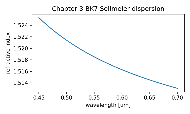
The curve slopes downward from blue to red.

The slope is gentle, but optical systems care about gentle slopes. A lens surface does not ask whether a number looks dramatic. It uses the number in Snell’s law. A tiny index difference becomes a tiny angular difference. After propagation, that angular difference becomes a longitudinal or transverse color error. Across multiple surfaces, it becomes part of the design problem.

This is why achromatic doublets exist. A single glass has dispersion. Pairing glasses with different dispersion properties allows a designer to reduce color error. We are not designing achromats yet, but the reason they exist is already visible in this curve.

Abbe number: a compact dispersion summary

Glass catalogs need a compact way to describe dispersion. One common summary is the Abbe number.

For the d-line convention:

V_d = (n_d - 1) / (n_F - n_C)

where:

n_d = refractive index at the helium d-line, about 587.6 nm
n_F = refractive index at the hydrogen F-line, about 486.1 nm
n_C = refractive index at the hydrogen C-line, about 656.3 nm

Optiland’s material API describes the same V_d definition using the d, F, and C spectral lines. (Optiland)

Let us compute it.

F_LINE_UM = 0.4861327
D_LINE_UM = 0.5875618
C_LINE_UM = 0.6562725

def abbe_number_vd(material):
    n_F = material.n(F_LINE_UM)
    n_d = material.n(D_LINE_UM)
    n_C = material.n(C_LINE_UM)
    return (n_d - 1.0) / (n_F - n_C)

print(abbe_number_vd(N_BK7))

For N-BK7, the result should be close to 64.17, depending on coefficient precision and rounding.

What does this number mean?

A higher Abbe number means lower dispersion. A lower Abbe number means stronger dispersion.

Crown glasses often have relatively high Abbe numbers. Flint glasses often have lower Abbe numbers and higher dispersion. That distinction is central to traditional color correction.

But we should be careful.

The Abbe number is a summary, not a full refractive-index model. It uses three wavelengths to describe a curve. That is useful for classification, comparison, and approximate modeling. It is not the same as having the full dispersion curve.

This is a recurring theme in optical computation:

A compact parameter is useful only if you remember what it compresses.

An Abbe number does not replace n(λ). It gives one important clue about it.

Wavelength sets and weights

A real optical design is usually not evaluated at only one wavelength.

A simple visible-light system may use three wavelengths:

blue:  0.4861 µm
green: 0.5876 µm
red:   0.6563 µm

A more realistic imaging design may use several wavelengths with weights. The weights tell the software how much each wavelength matters in a particular analysis or optimization.

A crude example:

wavelength [µm]   weight
0.4861            0.5
0.5876            1.0
0.6563            0.5

This does not mean the green ray is “more real.” It means the design evaluation gives more importance to that wavelength.

Weights can represent a simplified spectral distribution, sensor response, photopic eye response, design priority, or just a practical engineering choice. The meaning depends on the system.

For our teaching code, we can represent wavelengths like this:

from dataclasses import dataclass

@dataclass
class Wavelength:
    value_um: float
    weight: float = 1.0
    is_primary: bool = False

wavelengths = [
    Wavelength(0.4861327, weight=0.5),
    Wavelength(0.5875618, weight=1.0, is_primary=True),
    Wavelength(0.6562725, weight=0.5),
]

Then we can evaluate material indices:

for wl in wavelengths:
    n = N_BK7.n(wl.value_um)
    marker = " primary" if wl.is_primary else ""
    print(f"{wl.value_um:.7f} µm  weight={wl.weight:.2f}  n={n:.7f}{marker}")

This is a small data structure, but it is the beginning of polychromatic optical calculation.

Later, when we compute spot diagrams, we may trace rays at multiple wavelengths and plot them in different colors. When we compute MTF, we may compute a weighted polychromatic result. When we optimize a lens, the merit function may include errors at multiple wavelengths.

Again, the later plot begins here.

Updating the lens system from Chapter 2

In Chapter 2, our LensSystem stored wavelengths as a simple list of floats:

wavelengths_um = [0.5876]

Now we can be more explicit:

from dataclasses import dataclass, field
from typing import List, Optional
import math

@dataclass
class Wavelength:
    value_um: float
    weight: float = 1.0
    is_primary: bool = False

@dataclass
class Surface:
    radius: float
    thickness: float
    material_after: str = "air"
    semi_diameter: Optional[float] = None
    conic: float = 0.0
    is_stop: bool = False
    surface_type: str = "spherical"
    comment: str = ""

    @property
    def curvature(self):
        if math.isinf(self.radius):
            return 0.0
        return 1.0 / self.radius

@dataclass
class LensSystem:
    surfaces: List[Surface] = field(default_factory=list)
    wavelengths: List[Wavelength] = field(default_factory=list)
    units: str = "mm"

    def add_surface(self, surface):
        self.surfaces.append(surface)

    def add_wavelength(self, value_um, weight=1.0, is_primary=False):
        self.wavelengths.append(Wavelength(value_um, weight, is_primary))

Now we need a material library.

class MaterialLibrary:
    def __init__(self):
        self._materials = {}

    def add(self, name, material):
        self._materials[name] = material

    def n(self, name, wavelength_um):
        if name == "air":
            return 1.0

        if name not in self._materials:
            raise ValueError(f"Unknown material: {name}")

        return self._materials[name].n(wavelength_um)

Register N-BK7:

materials = MaterialLibrary()
materials.add("N-BK7", N_BK7)

Build the singlet again:

lens = LensSystem()

lens.add_surface(Surface(
    radius=float("inf"),
    thickness=float("inf"),
    material_after="air",
    surface_type="object",
    comment="object at infinity",
))

lens.add_surface(Surface(
    radius=+50.0,
    thickness=5.0,
    material_after="N-BK7",
    semi_diameter=10.0,
    is_stop=True,
    comment="front lens surface",
))

lens.add_surface(Surface(
    radius=-50.0,
    thickness=45.0,
    material_after="air",
    semi_diameter=10.0,
    comment="back lens surface",
))

lens.add_surface(Surface(
    radius=float("inf"),
    thickness=0.0,
    material_after="air",
    surface_type="image",
    comment="image plane",
))

lens.add_wavelength(0.4861327, weight=0.5)
lens.add_wavelength(0.5875618, weight=1.0, is_primary=True)
lens.add_wavelength(0.6562725, weight=0.5)

Now ask for material transitions at each physical surface and wavelength.

def material_before_after(lens, surface_index, starting_material="air"):
    if surface_index == 0:
        before = starting_material
    else:
        before = lens.surfaces[surface_index - 1].material_after

    after = lens.surfaces[surface_index].material_after
    return before, after

for wl in lens.wavelengths:
    print(f"\nWavelength {wl.value_um:.7f} µm")
    for i, surface in enumerate(lens.surfaces):
        if surface.surface_type in ("object", "image"):
            continue

        before, after = material_before_after(lens, i)
        n_before = materials.n(before, wl.value_um)
        n_after = materials.n(after, wl.value_um)

        print(
            f"surface {i}: {before:>6} n={n_before:.7f} "
            f"→ {after:>6} n={n_after:.7f}"
        )

This is still not ray tracing, but it is now ready for ray tracing.

At each surface, for each wavelength, the program can obtain n_before and n_after.

That is exactly what the refraction algorithm will need in Chapter 6.

Snell’s law is waiting for these numbers

We are not deriving vector refraction yet. That deserves its own chapter. But we can preview why the index function matters.

Scalar Snell’s law says:

n₁ sin θ₁ = n₂ sin θ₂

where:

n₁ = refractive index before the surface
n₂ = refractive index after the surface
θ₁ = incident angle relative to the surface normal
θ₂ = refracted angle relative to the surface normal

If n₂ changes with wavelength, then θ₂ changes with wavelength.

Let us compute a tiny example. Suppose a ray in air enters N-BK7 at an incident angle of 10 degrees.

import math

def refracted_angle_deg(theta1_deg, n1, n2):
    theta1 = math.radians(theta1_deg)
    s2 = n1 * math.sin(theta1) / n2

    if abs(s2) > 1.0:
        return None  # total internal reflection

    theta2 = math.asin(s2)
    return math.degrees(theta2)

theta1_deg = 10.0

for wl in [F_LINE_UM, D_LINE_UM, C_LINE_UM]:
    n2 = N_BK7.n(wl)
    theta2 = refracted_angle_deg(theta1_deg, n1=1.0, n2=n2)
    print(f"{wl:.7f} µm  n={n2:.7f}  theta2={theta2:.6f} degrees")

The differences in refracted angle will be small. That is fine. Small differences are real.

A lens contains curved surfaces. Rays enter at different heights. The local surface normal changes. The ray propagates after refraction. A small angular difference at one surface becomes a position difference at another surface or image plane.

This is the computational birth of chromatic aberration.

It does not appear later as a mysterious defect. It begins here:

n = n(λ)

Then Snell’s law uses that n.

Longitudinal color in one thin-lens approximation

A full chromatic focus calculation requires ray tracing or paraxial system calculation. We will learn both later. But a thin-lens preview can show the direction.

For a thin lens in air, a rough lensmaker-style relationship is:

1/f ≈ (n - 1) (1/R₁ - 1/R₂)

This simplified form ignores thickness and assumes the lens is in air. It is not enough for serious design, but it is enough to see the effect of dispersion.

If n changes with wavelength, then f changes with wavelength.

Let us compute that for a symmetric biconvex lens with:

R₁ = +50 mm
R₂ = -50 mm

def thin_lens_focal_length(n, R1, R2):
    power = (n - 1.0) * (1.0 / R1 - 1.0 / R2)
    return 1.0 / power

R1 = +50.0
R2 = -50.0

for wl in [F_LINE_UM, D_LINE_UM, C_LINE_UM]:
    n = N_BK7.n(wl)
    f = thin_lens_focal_length(n, R1, R2)
    print(f"{wl:.7f} µm  n={n:.7f}  f≈{f:.3f} mm")

You should see that the focal length is not exactly the same at all three wavelengths.

This is not our final model. It is a preview of a fact the ray tracer will later show in a more direct way:

A single-element lens does not bring all wavelengths to the same focus.

Now the cause is visible: the material curve enters the refraction calculation.

A material can also absorb light

So far, we have talked only about refractive index n.

Many material databases also describe extinction coefficient k, which relates to absorption. In a complex refractive index:

N = n + i k

the real part n controls phase velocity and refraction, while k describes loss.

For the geometric ray tracing chapters that come next, we will mostly use n. But it is useful to know that a richer material model may also know about absorption. Optiland’s material classes include both refractive-index and extinction-coefficient methods, and its material tutorial demonstrates computing both n and k versus wavelength. (Optiland)

We will not build absorption into the ray tracer yet. That would distract from the main chain. But when we later discuss transmission, coatings, or non-visible materials, k becomes part of the story.

For now:

ray direction calculation → needs n(λ)
absorption/transmission calculation → may need k(λ)

One thing at a time.

Optiland material models

Our teaching code has two material types:

ConstantMaterial
SellmeierMaterial

A real library needs more.

Current Optiland material documentation describes several material types, including IdealMaterial, AbbeMaterial, AbbeMaterialE, and Material; its Material class connects to data from refractiveindex.info, while IdealMaterial provides fixed-index behavior and AbbeMaterial provides a model based on refractive index and Abbe number. (Optiland)

A minimal Optiland-style material check can look like this:

import numpy as np
import matplotlib.pyplot as plt

from optiland.materials import IdealMaterial, AbbeMaterial, Material

# Fixed-index material.
ideal = IdealMaterial(n=1.5, k=0)

# Approximate glass model from n_d and Abbe number.
abbe_glass = AbbeMaterial(n=1.5168, abbe=64.17, model="buchdahl")

# Database-backed material lookup.
# Depending on installed version and database contents,
# specifying reference or catalog can help disambiguate the material.
bk7 = Material("N-BK7", reference="Schott")

wavelengths = np.linspace(0.45, 0.70, 200)

plt.plot(wavelengths, ideal.n(wavelengths), label="Ideal n=1.5")
plt.plot(wavelengths, abbe_glass.n(wavelengths), label="Abbe model")
plt.plot(wavelengths, bk7.n(wavelengths), label="N-BK7 database")

plt.xlabel("wavelength [µm]")
plt.ylabel("refractive index")
plt.title("Different material models")
plt.legend()
plt.show()

This code is not meant to replace our Sellmeier implementation. It shows the same idea at library level.

The pattern is consistent:

material object → n(wavelength)

That is the interface we want to understand.

The real library may use databases, fitted formulas, caching, search rules, and backend arrays. Our teaching class uses three coefficients and a square root. The difference is important in engineering, but the conceptual contract is the same.

Material belongs to the surface transition

Let us return to the prescription.

In a sequential lens table, the material listed at a surface normally describes the medium after that surface.

For the singlet:

surface 1: material_after = N-BK7
surface 2: material_after = air

At surface 1:

n_before = n_air(λ)
n_after  = n_N-BK7(λ)

At surface 2:

n_before = n_N-BK7(λ)
n_after  = n_air(λ)

This is one of the simplest places to make a wrong ray tracer.

If you accidentally use the same material on both sides, the ray will not bend. If you swap before and after, the ray may bend in the wrong direction. If you use a constant glass index, the system will not show chromatic behavior. If you pass wavelength in nanometers to a function expecting micrometers, the result may be nonsense.

So before writing the refraction function, it is worth making material transitions explicit.

def index_transition(lens, materials, surface_index, wavelength_um):
    before_name, after_name = material_before_after(lens, surface_index)
    n_before = materials.n(before_name, wavelength_um)
    n_after = materials.n(after_name, wavelength_um)
    return n_before, n_after

Then:

for i, surface in enumerate(lens.surfaces):
    if surface.surface_type in ("object", "image"):
        continue

    n1, n2 = index_transition(lens, materials, i, D_LINE_UM)
    print(f"surface {i}: n1={n1:.7f}, n2={n2:.7f}")

This function is small, but it protects the logic of the next chapters.

A ray tracer should not be guessing which index to use. The prescription and material library should answer that question.

Primary wavelength is not the only wavelength

Optical design software often marks one wavelength as primary.

The primary wavelength may be used for layout, focus, paraxial reference, or default analysis. But that does not mean the other wavelengths are decorative. They may be essential for evaluating chromatic correction.

A common beginner mistake is to see a primary wavelength and forget the rest.

Better wording is:

The primary wavelength is the reference wavelength.
The wavelength set describes the spectral conditions to evaluate.

In code:

def primary_wavelength(lens):
    primary = [wl for wl in lens.wavelengths if wl.is_primary]

    if len(primary) != 1:
        raise ValueError("Lens should have exactly one primary wavelength.")

    return primary[0]

print(primary_wavelength(lens))

That function seems almost too strict, but strictness is helpful here. Ambiguous optical settings lead to ambiguous results.

When we later compute a spot diagram, we can choose:

trace only primary wavelength
trace all wavelengths
trace all wavelengths with weights

Those are different analyses. The program should know which one it is doing.

Wavelength weights are not magic

Suppose an MTF plot is labeled “polychromatic.”

That sounds impressive, but it still has to mean something concrete.

At some point, the program has to combine information from multiple wavelengths. It may use weights. It may use a spectral distribution. It may use sensor response. It may use a simplified user-defined set.

A simple weighted average looks like this:

def weighted_average(values, weights):
    values = np.asarray(values, dtype=float)
    weights = np.asarray(weights, dtype=float)
    return np.sum(values * weights) / np.sum(weights)

For refractive index itself, averaging is not usually the right physical operation for a lens calculation, because rays at each wavelength should be traced with their own index. But the function shows the general idea of weighted combination.

A better mental model is:

for each wavelength:
    compute the optical result using n(λ)

then:
    combine wavelength-specific results according to the analysis method

That matters for later.

A polychromatic spot diagram is not created by tracing one average wavelength. It is created by tracing multiple wavelengths and displaying or combining their ray intersections. A polychromatic MTF is not made by pretending the glass has one average index. It requires wavelength-aware computation before the final combination.

This is a place where software commands can hide a lot.

The button may say:

Polychromatic MTF

The computation says:

wavelength set
→ material indices at each wavelength
→ ray or wavefront calculation at each wavelength
→ wavelength-specific image-quality result
→ weighted combination

We are not ready to compute that full chain yet. But now we know where it begins.

Common mistakes with materials and wavelengths

Let us collect the mistakes now, while they are still easy to see.

Mistake 1: Treating refractive index as a universal constant

N-BK7 ≈ 1.5168 is not a complete material model. It is a reference value near the d-line.

Use constant index when you intentionally want a simplified model. Do not use it accidentally.

Mistake 2: Passing wavelength in the wrong unit

A function expecting micrometers should receive:

0.5876

not:

587.6

unless the function explicitly expects nanometers.

This is one of the easiest ways to ruin a calculation quietly.

Mistake 3: Confusing Abbe number with full dispersion

The Abbe number summarizes dispersion using selected wavelengths. It is useful, but it is not the whole refractive-index curve.

Mistake 4: Forgetting that material is “after surface”

In a sequential prescription, the material listed at surface i usually describes the medium after surface i.

The refraction at a surface needs both sides:

previous material → current material_after

Mistake 5: Averaging refractive indices too early

For multi-wavelength analysis, do not replace all wavelengths with one average refractive index unless that is a deliberate approximation. Trace or compute each wavelength according to the analysis being performed.

Mistake 6: Ignoring valid wavelength range

Dispersion formulas are valid over specified wavelength ranges. Extrapolating outside that range can produce wrong results. Real material databases usually carry range information for a reason.

Mistake 7: Forgetting air is also a material

For many visible-light teaching examples, we treat air as n = 1.0. In high-precision work, air itself has wavelength-, temperature-, pressure-, and humidity-dependent refractive index. We will use 1.0 for now because it keeps the early ray tracer focused. But it is still a model choice.

What this chapter adds to the computation chain

In Chapter 2, we could say:

surface 1 has material N-BK7

Now we can say:

surface 1 changes the medium from air to N-BK7

at λ = 0.4861 µm:
    n_before = 1.0
    n_after  = n_N-BK7(0.4861)

at λ = 0.5876 µm:
    n_before = 1.0
    n_after  = n_N-BK7(0.5876)

at λ = 0.6563 µm:
    n_before = 1.0
    n_after  = n_N-BK7(0.6563)

That is a real improvement.

The prescription is no longer only geometry. It now contains wavelength-dependent optical behavior.

Our computational chain has become:

surface table
→ material names
→ material models
→ refractive index n(λ)
→ index transition at each surface
→ ready for Snell refraction

This is exactly the missing piece before we define rays.

A small final test

Let us write one compact test that confirms the chapter’s work.

def print_surface_indices(lens, materials):
    for wl in lens.wavelengths:
        print(f"\nλ = {wl.value_um:.7f} µm, weight = {wl.weight}")
        for i, s in enumerate(lens.surfaces):
            if s.surface_type in ("object", "image"):
                continue

            before, after = material_before_after(lens, i)
            n1 = materials.n(before, wl.value_um)
            n2 = materials.n(after, wl.value_um)

            print(
                f"surface {i}: {before} → {after}, "
                f"n1={n1:.7f}, n2={n2:.7f}"
            )

print_surface_indices(lens, materials)

If this prints different N-BK7 indices for different wavelengths, the material system is doing its job.

It is not tracing rays yet. It is preparing the numbers that ray tracing needs.

That is enough.

The road ahead

We now have:

a lens prescription as data
surface geometry
material names
wavelength settings
a refractive-index function n(λ)
index transitions at each surface

The next object is the ray itself.

A ray is not a vague line in a drawing. In code, it must have a position, a direction, a wavelength, perhaps intensity, perhaps status flags, and eventually optical path length. It must be able to propagate. It must be able to meet surfaces. It must carry the wavelength that tells the material library which refractive index to use.

So Chapter 4 will ask a plain question:

What is a ray in code?

Once we answer that, the pieces will begin to move.

The lens prescription gives the world.

The material model gives each medium its wavelength-dependent behavior.

The ray will be the traveler.

Generated validation figure

Source and validation note

The wavelength-dependent material discussion should be read against glass-catalog and optical-constants sources, not only against the simplified teaching code. In the companion validation, BK7 dispersion is generated for teaching purposes; production work should use a catalog source and record the exact glass vendor, reference data, wavelength unit, and temperature assumptions.