Chapter 2: What a Lens Prescription Really Is
A lens drawing is easy to like.
You see curved pieces of glass. You see air gaps. You see a stop. You may see rays bending through the system and meeting near an image plane. A drawing gives your eyes something to hold onto.
But a drawing is not what the optical software calculates from.
The software needs a prescription.
At first, a lens prescription looks disappointingly plain. It is usually a table: surface number, radius, thickness, material, aperture, maybe conic constant, maybe aspheric coefficients, maybe comments. Compared with a ray-traced layout or an MTF plot, it looks almost bureaucratic.
That plainness is the point.
A lens prescription is the optical system written as data.
Once the system is written as data, a program can do something with it. It can compute surface positions. It can ask where a ray intersects the next surface. It can look up refractive index at a wavelength. It can decide whether a ray is blocked by an aperture. It can trace many rays to an image plane. Later, it can build spot diagrams, wavefront maps, PSF images, and MTF curves.
So before we trace rays, before we calculate OPD, before we touch Fourier transforms, we need to learn a modest but crucial skill:
We need to read a lens prescription as a computational object.
This chapter is about that object.
Not about a beautiful optical layout. Not about final image quality. Just the data structure that makes all later calculations possible.
That may sound like a small step. It is not. If the prescription is unclear, everything downstream becomes unclear. A wrong surface radius, a misunderstood thickness, or a misplaced material assignment can quietly poison the entire calculation chain.
Here we can be explicit. We are not memorizing a professional lens design table; we are turning a piece of glass into data a Python program can use.
A prescription is a sequence
Most introductory optical drawings make a lens look like an object in space. A prescription makes it look like a sequence.
Light travels through one surface, then the next, then the next. In a sequential optical system, surfaces are ordered along the optical path. The program does not first see “a lens” in the human sense. It sees something more like this:
surface 0 → surface 1 → surface 2 → surface 3 → ...
Each surface tells the program:
Where am I?
What shape am I?
What medium comes after me?
How far is the next surface?
How large is the usable aperture here?
For a simple singlet lens, a minimal table might look like this:
surface   radius      thickness     material     semi-diameter     note
0         infinity    infinity      air          —                 object
1         +50.0       5.0           N-BK7        10.0              front lens surface
2         -50.0       45.0          air          10.0              back lens surface
3         infinity    0.0           air          —                 image plane
This is already enough to teach several important conventions.
The first row is often the object surface. If the object is at infinity, the radius and thickness may be represented as infinity. This does not mean the software is trying to draw an infinitely large surface. It means the incoming rays are treated according to an object-at-infinity convention.
Surface 1 is the first physical glass surface. Its radius is positive in this example. It has a thickness of 5.0, which means the distance from surface 1 to surface 2 along the optical axis is 5.0 units. If we use millimeters, then this is 5.0 mm.
The material listed at surface 1 is N-BK7. In the usual sequential prescription convention, this means the medium after surface 1 is N-BK7. In other words, once a ray crosses surface 1, it travels through N-BK7 until it reaches surface 2.
Surface 2 has material air, which means after crossing surface 2, the ray leaves the glass and travels in air toward the image plane.
Surface 3 is the image plane. It is still treated as a surface in the sequence, even though it may not be a physical piece of glass.
This is the first useful mental shift:
The image plane is not just “where the drawing ends.” In computation, it is another target surface where ray positions can be evaluated.
That is how a spot diagram eventually becomes possible. The program traces rays through the earlier surfaces, then asks where they land on the image surface.
The main columns
Let us unpack the common columns one by one.
A basic lens prescription often includes these fields:
radius
thickness
material
semi-diameter
conic constant
surface type
Professional software may include many more: coating, aperture type, solve type, pickup, coordinate break, aspheric coefficients, diffractive terms, thermal model, tolerance data, and so on. We do not need all of that yet.
For now, the six fields above are enough to build the first data structure.
Radius: the surface curvature in human form
The radius tells us how curved a surface is.
For a spherical surface, the radius is the radius of the sphere from which the surface is cut. A large radius means a gentle surface. An infinite radius means a plane. A small radius means a stronger curve.
In many optical prescriptions, the radius is signed. The sign convention depends on the coordinate system, and different tools may define signs carefully in their own way. In this book, we will use the common sequential optics intuition: light travels roughly in the positive z direction, and the sign of the radius tells us where the center of curvature lies relative to the surface vertex.
For now, do not let the sign convention become a monster under the bed. We will make it explicit in code whenever it matters.
A radius is often converted into curvature:
c = 1 / R
If R is infinite, the curvature is zero. That is exactly what we want for a plane surface.
This small conversion is common because many equations are cleaner when written in terms of curvature c rather than radius R.
In code, we should handle infinity gently. A plane surface should not cause a divide-by-infinity surprise or a special-case disaster. We can write a helper function:
import math

def curvature_from_radius(radius):
    """Return curvature c = 1/R, with planes represented by c = 0."""
    if math.isinf(radius):
        return 0.0
    return 1.0 / radius

print(curvature_from_radius(50.0))        # 0.02
print(curvature_from_radius(float("inf"))) # 0.0
This is not glamorous code. But it is exactly the kind of small convention that keeps an optical program sane.
Thickness: distance to the next surface
Thickness is one of the most easily misunderstood columns.
In a sequential prescription, thickness usually means:
the axial distance from this surface to the next surface.
It does not mean “the thickness of this surface.” A mathematical surface has no thickness. It is a boundary. The thickness column tells us how far to move before reaching the next boundary.
For a physical lens element, the thickness after the first surface is often the glass center thickness. For an air gap, the thickness after the second surface may be the distance through air to the next optical element or image plane.
In our simple singlet:
surface 1 thickness = 5.0
means the axial distance from the front glass surface to the back glass surface is 5.0 mm.
surface 2 thickness = 45.0
means the axial distance from the back glass surface to the image plane is 45.0 mm.
This convention matters because it defines the global positions of the surfaces.
If surface 1 is at z = 0, then surface 2 is at z = 5, and surface 3 is at z = 50.
That is already a little optical system in coordinates.
Let us compute those positions.
from dataclasses import dataclass
from typing import Optional
import math

@dataclass
class Surface:
    radius: float
    thickness: float
    material_after: str = "air"
    semi_diameter: Optional[float] = None
    conic: float = 0.0
    comment: str = ""

def surface_vertices(surfaces):
    """Return the z-coordinate of each surface vertex."""
    z = 0.0
    vertices = []

    for s in surfaces:
        vertices.append(z)

        # The last image surface may have thickness 0.
        # An infinite object thickness should not move our finite drawing origin.
        if not math.isinf(s.thickness):
            z += s.thickness

    return vertices

surfaces = [
    Surface(radius=float("inf"), thickness=float("inf"), comment="object at infinity"),
    Surface(radius=+50.0, thickness=5.0, material_after="N-BK7",
            semi_diameter=10.0, comment="front lens surface"),
    Surface(radius=-50.0, thickness=45.0, material_after="air",
            semi_diameter=10.0, comment="back lens surface"),
    Surface(radius=float("inf"), thickness=0.0, material_after="air",
            comment="image plane"),
]

# For a simple finite layout, we usually start drawing at the first physical surface.
finite_surfaces = surfaces[1:]
for i, (s, z) in enumerate(zip(finite_surfaces, surface_vertices(finite_surfaces)), start=1):
    print(i, z, s.comment)
This prints surface positions for the finite part of the system. We skipped the object-at-infinity row when computing drawing coordinates, because it is a boundary condition, not a finite physical surface.
Already, the prescription has become something a program can inspect.
Material: the medium after the surface
The material column tells us what medium the ray enters after crossing a surface.
This is worth repeating because it is a common source of mistakes:
In a sequential prescription, material usually belongs to the space after the surface, not before it.
For surface 1 in the singlet, the material after the surface is glass. For surface 2, the material after the surface is air.
That means each surface interaction needs two refractive indices:
n_before → n_after
At surface 1, for a ray entering the lens:
air → N-BK7
At surface 2:
N-BK7 → air
We will not calculate refraction in this chapter. That comes later. But the prescription already contains the information needed for it.
For now, we can add a very small material model. It will not handle real dispersion yet. Chapter 3 will handle wavelength and refractive index more carefully. Here, we only want the data structure to know that different media exist.
SIMPLE_INDEX = {
    "air": 1.0,
    "N-BK7": 1.5168,  # approximate value near the yellow helium d-line
}

def refractive_index(material_name, wavelength_um=0.5876):
    """A placeholder material model.

    Chapter 3 will replace this with wavelength-dependent glass behavior.
    """
    try:
        return SIMPLE_INDEX[material_name]
    except KeyError:
        raise ValueError(f"Unknown material: {material_name}")

def media_before_after(surfaces, surface_index, starting_material="air"):
    """Return material before and after a surface in a sequential system."""
    if surface_index == 0:
        before = starting_material
    else:
        before = surfaces[surface_index - 1].material_after

    after = surfaces[surface_index].material_after
    return before, after

for i, s in enumerate(finite_surfaces):
    before, after = media_before_after(finite_surfaces, i)
    print(f"Surface {i+1}: {before} -> {after}")
A real optical library will use a glass catalog and compute refractive index as a function of wavelength. Our placeholder is deliberately simple. It is a signpost, not a finished material engine.
The important point is structural:
Refraction later depends on material transitions that are already encoded in the prescription.
Semi-diameter: the usable size of the surface
The semi-diameter is the usable radius of the surface aperture. If the semi-diameter is 10 mm, the clear circular region has a diameter of 20 mm.
It is tempting to treat semi-diameter as merely a drawing parameter. Do not do that. It is also a ray-blocking parameter.
A ray may geometrically intersect a spherical surface, but if the intersection point lies outside the usable semi-diameter, the ray should be considered blocked or invalid for that surface.
In a simple circular aperture check:
sqrt(x² + y²) <= semi_diameter
or, more efficiently:
x² + y² <= semi_diameter²
In code:
def inside_clear_aperture(x, y, semi_diameter):
    if semi_diameter is None:
        return True
    return x*x + y*y <= semi_diameter*semi_diameter

print(inside_clear_aperture(3.0, 4.0, 5.0))  # True
print(inside_clear_aperture(6.0, 0.0, 5.0))  # False
This tiny check will matter later when we trace a bundle of rays. Some rays will pass through the clear aperture. Some will be clipped. The final spot diagram, illumination pattern, PSF, and MTF can all be affected by aperture definitions.
Again, the later plot begins here, in the plain table.
Stop surface: the aperture that controls the beam
Not every semi-diameter is the aperture stop.
Every surface may have a clear aperture, but the aperture stop is the element that limits the cone of rays through the system. In many optical systems, the stop may be a physical diaphragm. In simple examples, a lens surface itself may be marked as the stop.
A prescription often marks one surface as the stop:
surface 1: is_stop = True
This is not just a note for drawing. The stop helps determine entrance pupil, exit pupil, ray sampling, F-number, and which rays are considered part of the imaging bundle.
For now, we can add an is_stop field to our Surface class.
@dataclass
class Surface:
    radius: float
    thickness: float
    material_after: str = "air"
    semi_diameter: Optional[float] = None
    conic: float = 0.0
    is_stop: bool = False
    comment: str = ""
This does not yet calculate pupils. It simply records the information. Later chapters will use it.
This is a recurring pattern in computational optics:
record the optical data first
then write algorithms that consume that data
If the data structure is vague, the algorithms become a mess.
Conic constant: the first step beyond spheres
A sphere is not the only useful optical surface.
Many lenses use conic or aspheric surfaces to control aberrations. The conic constant describes how the surface deviates from a sphere into shapes such as paraboloids, ellipsoids, or hyperboloids.
The sag of a rotationally symmetric conic surface can be written as:
z(r) = (c r²) / (1 + sqrt(1 - (1 + k)c²r²))
where:
r = sqrt(x² + y²)
c = 1 / R
k = conic constant
For a sphere, k = 0.
At this point, you do not need to memorize the sag equation. Just see what it does. It turns a surface prescription into a height function. Given a radial distance r from the optical axis, it tells us the z sag of the surface relative to its vertex.
This matters because ray-surface intersection eventually asks:
Where does the ray meet this actual surface shape?
For this chapter, we will only evaluate the sag. We will not solve full ray-asphere intersections yet.
import numpy as np

def conic_sag(r, radius, conic=0.0):
    """Sag z(r) for a rotationally symmetric conic surface."""
    if math.isinf(radius):
        return np.zeros_like(r, dtype=float)

    c = 1.0 / radius
    inside = 1.0 - (1.0 + conic) * (c * r)**2

    # Numerical guard for values very close to zero.
    inside = np.maximum(inside, 0.0)

    return (c * r**2) / (1.0 + np.sqrt(inside))

r = np.linspace(0.0, 10.0, 6)
print(conic_sag(r, radius=50.0, conic=0.0))
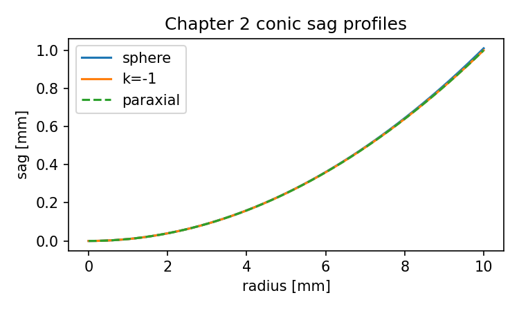
The output values are small near the axis and grow toward the edge. That is the surface becoming curved.
If you want to visualize it:
import matplotlib.pyplot as plt

r = np.linspace(0.0, 10.0, 200)

plt.plot(r, conic_sag(r, radius=50.0, conic=0.0), label="sphere, R=50")
plt.plot(r, conic_sag(r, radius=50.0, conic=-1.0), label="paraboloid-like, k=-1")
plt.xlabel("radial coordinate r [mm]")
plt.ylabel("sag z [mm]")
plt.title("Conic sag profiles")
plt.legend()
plt.show()
This is a quiet but important moment. A row in a table has become a mathematical surface. The surface has become a function. A function can be evaluated. Later, a ray can intersect it.
That is how the black box starts opening.
Surface type: plane, sphere, conic, asphere
The surface type tells the program what geometry model to use.
A minimal program may support only:
plane
sphere
A practical design tool may support:
standard spherical surface
conic surface
even asphere
odd asphere
toroidal surface
freeform surface
coordinate break
diffractive surface
mirror
image surface
Each type implies different geometry and different intersection logic.
This is why a surface data structure should not only store numbers. It should also store what those numbers mean.
For our teaching code, we can start with:
@dataclass
class Surface:
    radius: float
    thickness: float
    material_after: str = "air"
    semi_diameter: Optional[float] = None
    conic: float = 0.0
    is_stop: bool = False
    surface_type: str = "spherical"
    comment: str = ""
If surface_type is "spherical" and the radius is infinite, we can treat it as a plane. If it is "image", we know it is the final evaluation plane. A richer program would use separate classes for different surface types. For teaching, a field is enough.
Chapter 2 is not about perfect optical software architecture. It is about making the computational meaning visible.
A complete minimal prescription object
Now we can gather the pieces.
A lens system is more than a list of surfaces. It also has system-level settings:
aperture definition
field points
wavelengths
units
The surfaces describe the sequential geometry. The system settings describe how we illuminate and evaluate the system.
Let us write a small LensSystem.
from dataclasses import dataclass, field
from typing import List, Optional
import math

@dataclass
class Surface:
    radius: float
    thickness: float
    material_after: str = "air"
    semi_diameter: Optional[float] = None
    conic: float = 0.0
    is_stop: bool = False
    surface_type: str = "spherical"
    comment: str = ""

    @property
    def curvature(self):
        if math.isinf(self.radius):
            return 0.0
        return 1.0 / self.radius

@dataclass
class LensSystem:
    surfaces: List[Surface] = field(default_factory=list)
    aperture_type: str = "EPD"
    aperture_value: float = 10.0
    field_type: str = "angle"
    fields: List[float] = field(default_factory=lambda: [0.0])
    wavelengths_um: List[float] = field(default_factory=lambda: [0.5876])
    units: str = "mm"

    def add_surface(self, surface: Surface):
        self.surfaces.append(surface)

    def finite_vertices(self):
        """Return z positions for finite surfaces after skipping object at infinity."""
        finite = self.surfaces

        if finite and math.isinf(finite[0].thickness):
            finite = finite[1:]

        z = 0.0
        vertices = []
        for s in finite:
            vertices.append(z)
            if not math.isinf(s.thickness):
                z += s.thickness
        return vertices

    def print_prescription(self):
        print(" idx | radius | curvature | thickness | material | semi-dia | stop | comment")
        print("-----+--------+-----------+-----------+----------+----------+------+---------")
        for i, s in enumerate(self.surfaces):
            sd = "" if s.semi_diameter is None else f"{s.semi_diameter:.3g}"
            print(
                f"{i:>4} | "
                f"{s.radius:>7g} | "
                f"{s.curvature:>9.4g} | "
                f"{s.thickness:>9g} | "
                f"{s.material_after:>8} | "
                f"{sd:>8} | "
                f"{str(s.is_stop):>4} | "
                f"{s.comment}"
            )
Now define our singlet:
lens = LensSystem(aperture_type="EPD", aperture_value=10.0)

lens.add_surface(Surface(
    radius=float("inf"),
    thickness=float("inf"),
    material_after="air",
    surface_type="object",
    comment="object at infinity"
))

lens.add_surface(Surface(
    radius=+50.0,
    thickness=5.0,
    material_after="N-BK7",
    semi_diameter=10.0,
    is_stop=True,
    comment="front lens surface"
))

lens.add_surface(Surface(
    radius=-50.0,
    thickness=45.0,
    material_after="air",
    semi_diameter=10.0,
    comment="back lens surface"
))

lens.add_surface(Surface(
    radius=float("inf"),
    thickness=0.0,
    material_after="air",
    surface_type="image",
    comment="image plane"
))

lens.print_prescription()

print("\nFinite surface vertex positions:")
for z in lens.finite_vertices():
    print(z)
This is not yet ray tracing. It is something more basic:
It is a computable description of the optical system.
That description now contains the minimum information needed for later algorithms.
Chapter 3 will improve the material model. Chapter 4 will define rays. Chapter 5 will use the surface geometry to calculate intersections. Chapter 6 will use material transitions to calculate refraction.
The chain is already visible.
Why object and image are also surfaces
Beginners often want to remove the object and image rows because they are not physical lens elements.
Please resist that urge.
In sequential optics, object and image surfaces are useful because they make the system uniform. They let the program treat the optical path as a sequence with a beginning and an end.
The object surface defines how rays start. If the object is at infinity, rays from an on-axis field point enter parallel to the optical axis. If the object is finite, rays may start from a finite object height.
The image surface defines where rays are evaluated. A spot diagram is built from ray coordinates at the image surface. A focus shift can be represented by moving the image surface. Optimization may vary the final thickness to improve image quality.
So even when these rows look artificial, they serve a computational purpose.
They answer two questions:
How do rays enter the system?
Where do we measure their result?
Without those two answers, the lens is just glass floating in space.
The prescription is not the picture
Let us make this distinction very clear.
A prescription table can produce a drawing, but it is not the same thing as a drawing.
The drawing is a visualization derived from the data. The prescription is the data.
This matters because a drawing may hide details. It may not show exact radii. It may exaggerate shapes for readability. It may omit aperture limits or conic terms. It may not show wavelength, field, or material dispersion. A prescription, if complete, stores the details needed for computation.
In code, a drawing call should come after the data has been built:
prescription data → layout drawing
not the other way around.
This may feel obvious, but it saves confusion later. When software draws a lens, the drawing is not the source of truth. The source of truth is the optical model behind the drawing.
Optiland version of the same idea
Our small Python structure is useful because it exposes the skeleton. A real optical design library needs a more complete model.
Optiland’s documentation presents the Optic class as the primary interface for defining optical systems and describes surfaces as building blocks for optical elements. Its beginner example constructs a singlet by adding surfaces, setting an aperture, adding a field, adding a wavelength, drawing the system, and tracing rays. (Optiland) The current cheat sheet shows the same surface-by-surface pattern: create an optic.Optic(), add object, lens, and image surfaces, set entrance pupil diameter, field type, and wavelength. (Optiland)
A compact Optiland version of our singlet looks like this:
from optiland import optic

lens = optic.Optic()

# Object surface: object at infinity.
lens.surfaces.add(
    index=0,
    radius=float("inf"),
    thickness=float("inf")
)

# Front surface of the singlet.
# The material is the medium after this surface.
lens.surfaces.add(
    index=1,
    radius=50.0,
    thickness=5.0,
    material="N-BK7",
    is_stop=True
)

# Back surface of the singlet.
# After this surface, rays travel in air.
lens.surfaces.add(
    index=2,
    radius=-50.0,
    thickness=45.0
)

# Image surface.
lens.surfaces.add(index=3)

# System-level settings.
lens.set_aperture(aperture_type="EPD", value=10.0)
lens.fields.set_type("angle")
lens.fields.add(y=0.0)
lens.wavelengths.add(value=0.5876, is_primary=True)

lens.draw(num_rays=5)
Do not rush past this code.
It is doing the same conceptual work as our teaching structure. It creates a sequential optical system. It adds surfaces. It assigns material after a surface. It identifies a stop. It sets aperture, field, and wavelength. Then it draws the system.
The Optiland code is shorter because the library already knows how to organize optical objects. Our teaching code is more explicit because we want to see the bones.
Both are useful.
If we only use the teaching code, we risk building a toy world that never touches real optical software practice.
If we only use Optiland calls, we risk replacing one black box with another.
So we will keep both rails.
What the Optiland call hides on purpose
When we write:
lens.surfaces.add(index=1, radius=50.0, thickness=5.0, material="N-BK7")
a lot is being delegated.
The library must store the surface. It must decide how to represent the geometry. It must connect this surface to the next one. It must know how to look up the material later. It must participate in drawing, ray tracing, paraxial analysis, and optimization.
That is good software design. A library should not make the user manually wire every internal detail.
But as learners, we should still ask:
What does this one line imply?
It implies a surface vertex. It implies curvature. It implies a medium transition. It implies a distance to the next surface. It implies future ray-surface intersection. It implies future refraction.
A short API call is not a small optical event. It is a compact representation of many later computations.
That is the exact habit we are trying to build.
A small prescription reader
Professional lens files have their own formats. We will not build a full file parser here. But it is useful to see how close a prescription table is to code.
Suppose we write the surface data as a list of dictionaries:
raw_prescription = [
    {
        "radius": float("inf"),
        "thickness": float("inf"),
        "material_after": "air",
        "surface_type": "object",
        "comment": "object at infinity",
    },
    {
        "radius": 50.0,
        "thickness": 5.0,
        "material_after": "N-BK7",
        "semi_diameter": 10.0,
        "is_stop": True,
        "comment": "front lens surface",
    },
    {
        "radius": -50.0,
        "thickness": 45.0,
        "material_after": "air",
        "semi_diameter": 10.0,
        "comment": "back lens surface",
    },
    {
        "radius": float("inf"),
        "thickness": 0.0,
        "material_after": "air",
        "surface_type": "image",
        "comment": "image plane",
    },
]
Then build a LensSystem:
def build_lens_from_dicts(rows):
    lens = LensSystem()
    for row in rows:
        lens.add_surface(Surface(
            radius=row["radius"],
            thickness=row["thickness"],
            material_after=row.get("material_after", "air"),
            semi_diameter=row.get("semi_diameter"),
            conic=row.get("conic", 0.0),
            is_stop=row.get("is_stop", False),
            surface_type=row.get("surface_type", "spherical"),
            comment=row.get("comment", ""),
        ))
    return lens

lens = build_lens_from_dicts(raw_prescription)
lens.print_prescription()
This is simple, but the meaning is large.
A lens prescription can be stored, loaded, transformed, checked, drawn, traced, optimized, and compared.
That is why optical design software begins with tables. Tables are not an old-fashioned interface choice. They are a natural way to expose a sequential model.
Sanity checks before tracing rays
Before a program traces even one ray, it should check the prescription for obvious problems.
For example:
Is there at least one surface?
Is there an image surface?
Is there a stop or aperture definition?
Are finite thicknesses non-negative?
Are materials known?
Are semi-diameters positive when present?
Let us write a few simple checks.
def validate_lens(lens):
    errors = []

    if not lens.surfaces:
        errors.append("Lens has no surfaces.")

    if lens.surfaces and lens.surfaces[-1].surface_type != "image":
        errors.append("Last surface is not marked as an image surface.")

    if not any(s.is_stop for s in lens.surfaces):
        errors.append("No stop surface is marked.")

    for i, s in enumerate(lens.surfaces):
        if not math.isinf(s.thickness) and s.thickness < 0:
            errors.append(f"Surface {i} has negative thickness.")

        if s.semi_diameter is not None and s.semi_diameter <= 0:
            errors.append(f"Surface {i} has non-positive semi-diameter.")

        if s.material_after not in SIMPLE_INDEX:
            errors.append(f"Surface {i} uses unknown material: {s.material_after}")

    return errors

errors = validate_lens(lens)

if errors:
    print("Prescription problems:")
    for e in errors:
        print("-", e)
else:
    print("Prescription looks usable for the next step.")
This code does not prove the optical design is good. It only checks whether the data is internally usable.
That distinction is important.
A valid prescription may describe a terrible lens. It may produce huge aberrations. It may not focus where you expect. It may clip too many rays. It may have poor MTF.
But before we can judge performance, the system must at least be well-defined enough to calculate.
Drawing from the prescription
A rough 2D drawing can be produced from the prescription. We will not make a professional layout plot here, but even a simple sketch can help confirm that the signs and positions are not absurd.
For now, we can draw only the sag profiles of the two lens surfaces.
import numpy as np
import matplotlib.pyplot as plt

def plot_simple_lens(lens):
    finite_surfaces = lens.surfaces[1:] if math.isinf(lens.surfaces[0].thickness) else lens.surfaces
    z_vertices = lens.finite_vertices()

    for s, z0 in zip(finite_surfaces, z_vertices):
        if s.surface_type == "image":
            y = np.linspace(-12, 12, 2)
            z = np.full_like(y, z0)
            plt.plot(z, y, linestyle="--", label="image plane")
            continue

        if s.semi_diameter is None:
            continue

        y = np.linspace(-s.semi_diameter, s.semi_diameter, 200)
        r = np.abs(y)
        sag = conic_sag(r, s.radius, s.conic)

        # This simple plot assumes sag is measured along +z from the vertex.
        # Later chapters will handle sign conventions more carefully.
        z = z0 + sag
        plt.plot(z, y, label=s.comment or "surface")

    plt.gca().set_aspect("equal", adjustable="box")
    plt.xlabel(f"z [{lens.units}]")
    plt.ylabel(f"y [{lens.units}]")
    plt.title("Very simple lens layout from prescription data")
    plt.legend()
    plt.show()

plot_simple_lens(lens)
This plotting function is intentionally limited. It does not handle all sign conventions correctly for every possible surface. It does not draw glass fill regions. It does not trace rays. It is only a first confirmation that the prescription has geometric content.
And that is enough for this chapter.
When you run a mature optical package and call draw(), you are seeing a much more capable version of the same idea:
surface data → surface geometry → plotted layout
The drawing follows the prescription.
Units: the quiet source of many errors
Optical prescriptions usually use millimeters for distances and micrometers for wavelengths, but you should never assume silently.
A system may store:
surface radii in mm
thicknesses in mm
semi-diameters in mm
wavelengths in µm
spatial frequency in cycles/mm
That mixture is normal, but it demands attention.
If you use 0.5876 as a wavelength, do you mean millimeters, micrometers, or nanometers? In many optical design contexts, 0.5876 means micrometers. But in raw Python, a number has no unit. It is just a float.
So the data structure should either store units explicitly or follow a clear convention.
Our LensSystem stores:
units = "mm"
wavelengths_um = [0.5876]
That is a small act of kindness toward future readers, including future you.
Chapter 14 will return to units with more force, because PSF and MTF calculations are especially easy to damage with unit mistakes. For now, we only need the habit:
Never let a naked number pretend to be self-explanatory.
Common mistakes when reading prescriptions
Let us collect a few mistakes early, before they become expensive.
Mistake 1: Thinking material belongs to the surface itself
A surface is a boundary. The material column usually describes the medium after that boundary.
This affects refraction. At each surface, you need the index before and after the surface.
Mistake 2: Thinking thickness is the physical thickness of every row
Thickness is distance to the next surface. Sometimes that is glass center thickness. Sometimes it is an air gap. Sometimes it is distance to the image plane.
Mistake 3: Treating infinity as a normal huge number
An infinite radius means plane. An infinite object distance means object-at-infinity behavior. These are conventions and should be handled deliberately.
Do not replace infinity with a random large number unless you know exactly why you are doing it.
Mistake 4: Ignoring sign conventions
Radius sign, propagation direction, surface normal direction, and sag sign are connected. A sign mistake can create a system that looks plausible but refracts incorrectly.
We will keep sign conventions explicit in the ray-tracing chapters.
Mistake 5: Confusing semi-diameter with entrance pupil diameter
A surface semi-diameter is the usable radius of that surface. Entrance pupil diameter is a system-level aperture quantity. They are related in some systems, but they are not the same concept.
Mistake 6: Forgetting field and wavelength
A prescription without field and wavelength settings is incomplete for many analyses. You may have described the glass and surfaces, but not yet described how the system is used.
A ray trace needs rays. Rays depend on field and aperture sampling. Refraction depends on wavelength. Later image quality calculations depend on both.
Why this chapter matters for MTF
It may feel like we have traveled far away from MTF. We have not.
The MTF curve at the end of the book depends on all of these early choices.
Radius affects refraction. Thickness affects propagation distance. Material affects refractive index. Semi-diameter and stop affect which rays pass. Field defines the viewing direction. Wavelength changes phase and refraction. The image surface defines where results are measured.
That means the MTF curve is already being shaped here, long before we calculate Fourier transforms.
This is one of the central lessons of computational optics:
Image quality metrics are downstream results. The upstream data matters.
When a software package produces an MTF plot, it is not evaluating an abstract “lens.” It is evaluating a specific prescription under specific system settings.
So if you ever see an MTF plot without knowing the prescription, wavelength, field, aperture, focus position, and calculation method, you are seeing a result with most of its context removed.
Sometimes that is fine for a quick visual comparison. It is not fine for understanding.
What we have built
We now have a small but meaningful optical model.
It can store:
surface radius
thickness to next surface
material after surface
semi-diameter
conic constant
stop flag
surface type
aperture setting
field setting
wavelength setting
units
It can compute:
curvature from radius
finite surface vertex positions
simple conic sag values
basic aperture checks
basic prescription validation
It can also be compared with the way a real library like Optiland builds an optical system surface by surface.
That is enough to move to the next question.
Right now, our material model is almost embarrassingly simple. It says N-BK7 has one refractive index and leaves it there. Real glass does not behave that way. A lens bends blue light differently from red light. The same prescription evaluated at different wavelengths can focus differently and produce different aberrations.
So Chapter 3 will take the next step:
What does the material column really mean when refractive index depends on wavelength?
Once we answer that, the prescription will no longer be just geometry. It will become an optical system with color-dependent behavior.
And then, finally, we will be ready to define a ray.
Generated validation figure
Source and validation note
The prescription vocabulary in this chapter follows standard lens-design practice: radius, thickness, material, aperture, field, wavelength, conic data, and image surface settings. The simple teaching prescription is not a manufacturing prescription. Its purpose is to make the data model inspectable before full ray tracing begins. For the full publication bibliography, see appendices/SOURCES_AND_FURTHER_READING.md.