Chapter 1: Why MTF Does Not Come from a Software Button
A lens design program can make optics feel deceptively simple.
You build a lens. You enter a few radii, thicknesses, glasses, wavelengths, and field points. You click a button. A plot appears.
Maybe it is a spot diagram. Maybe it is a ray fan. Maybe it is a wavefront map. Or maybe it is the plot that many optical designers look at with a special mix of hope and dread: the MTF curve.
The curve looks authoritative. It has axes. It has sagittal and tangential lines. It has spatial frequency on one side and modulation on the other. If the lines stay high, the design looks promising. If they fall too early, something is wrong. The plot seems to speak in a clean engineering language:
This lens preserves contrast well.
This lens loses contrast at fine detail.
This field point is worse than the center.
This wavelength behaves differently.
This design is not ready yet.
That is all useful. But here is the problem.
Seeing an MTF curve is not the same as understanding where it came from.
This is not a complaint about optical design software. Good software hides labor, and in production work that is a gift. You do not want to manually compute every ray-surface intersection each time you adjust a radius. You do not want to write your own FFT every time you inspect diffraction performance. You want the tool to do those calculations quickly and reliably.
But learning is different from production.
For learning, the same convenience can become a wall. The software gives you the result, but the middle of the calculation disappears. You may learn to recognize a good MTF curve without knowing how that curve was built. You may know that PSF means point spread function, that OPD means optical path difference, and that MTF means modulation transfer function, but still not know how a lens prescription turns into those quantities.
That gap is the subject of this book.
We are going to open the box.
Not all at once. That would be unfair. The box contains geometry, vector math, ray tracing, first-order optics, wavefronts, sampling, Fourier transforms, normalization, units, and optimization. If we throw all of that at the reader in the first chapter, we have not taught anything. We have merely replaced one black box with another, more frightening one.
So we will begin with the map.
The curve that appears after you click the MTF button is not created by the button. It is the endpoint of a computation chain:
lens prescription
→ surfaces and materials
→ real ray tracing
→ paraxial reference
→ pupil sampling
→ optical path difference
→ pupil function
→ point spread function
→ optical transfer function
→ modulation transfer function
You do not need to understand every step yet. For now, just notice the shape of the chain. MTF sits near the end. It is not an isolated measurement floating above the optical system. It depends on the lens geometry, the glass, the wavelength, the aperture, the field point, the image plane, the wavefront error, and the numerical sampling method.
This is why a single MTF curve can be both powerful and dangerous.
Powerful, because it compresses many effects into one readable plot.
Dangerous, because the compression can make you forget the machinery underneath.
The curve is a consequence, not a starting point
Let us say we have a lens.
At the software level, the lens may appear as a table:
surface   radius      thickness     material     semi-diameter
0         infinity    infinity      air          —
1         50.0        5.0           N-BK7        10.0
2        -50.0        45.0          air          10.0
3         infinity    0.0           image        —
This is not just bookkeeping. It is the beginning of a computation.
Each row tells the program what kind of surface a ray may meet, where that surface is, how the ray should bend after reaching it, and where the next surface waits. A real optical design may contain many more surfaces, non-spherical shapes, apertures, solves, coatings, aspheric terms, multiple configurations, and multiple wavelengths. But the basic idea is the same:
A lens is not only a drawing. It is a structured set of inputs for calculation.
That is the first habit we need to build.
When you see a lens layout, ask: what data produced it?
When you see a ray trace, ask: how were the rays represented?
When you see a spot diagram, ask: where did those points come from?
When you see an MTF curve, ask: what chain of calculations created it?
This habit is more important than any single formula in the opening chapter. Formulae are easier to learn once you know where they belong.
A tiny preview of the computation chain
Before we touch a real optical system, let us look at a deliberately small piece of the chain.
In later chapters, we will compute wavefront error from traced rays. We will not cheat. We will build the ray model, intersect surfaces, refract directions, compare real rays to a reference, and construct OPD over the pupil.
For now, we will start halfway down the chain. Suppose we already have a pupil function. That means we know two things across the exit pupil:
- where light is allowed to pass;
- what phase delay the optical system has given to that light.
In scalar Fourier optics, a simplified pupil function can be written as:
P(x, y) = A(x, y) exp(i 2π W(x, y))
Here A(x, y) is the aperture amplitude mask. It may be 1 inside the pupil and 0 outside. W(x, y) is wavefront error measured in waves. The exponential turns wavefront error into optical phase.
Do not worry if this feels too fast. We will return to this carefully in the wavefront chapters. Right now, we only want to see that the PSF and MTF are not mystical objects. They can be computed.
Here is a minimal Python preview:
import numpy as np
import matplotlib.pyplot as plt

# A small square computational grid.
N = 256
u = np.linspace(-1.0, 1.0, N)
X, Y = np.meshgrid(u, u)
rho = np.sqrt(X**2 + Y**2)

# Circular pupil: light passes inside the unit circle.
aperture = rho <= 1.0

# A toy wavefront error in waves.
# This is not a full lens model yet. It is only a simple phase pattern.
defocus_waves = 0.5
W = defocus_waves * (2.0 * rho**2 - 1.0)

# Pupil function: amplitude mask times phase.
pupil = aperture * np.exp(1j * 2.0 * np.pi * W)

# PSF: squared magnitude of the Fourier transform of the pupil function.
amplitude = np.fft.fftshift(np.fft.fft2(np.fft.ifftshift(pupil)))
psf = np.abs(amplitude) ** 2
psf = psf / psf.sum()

# OTF: Fourier transform of the PSF.
otf = np.fft.fftshift(np.fft.fft2(np.fft.ifftshift(psf)))

# MTF: normalized magnitude of the OTF.
mtf = np.abs(otf)
mtf = mtf / mtf.max()

# A simple horizontal slice through the MTF.
center = N // 2
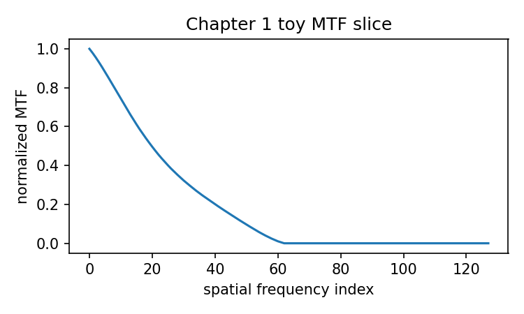
plt.plot(mtf[center, :])
plt.xlabel("sample index")
plt.ylabel("normalized modulation")
plt.title("A toy MTF slice from a toy pupil function")
plt.show()
This code is not yet a lens design program. It has no glass catalog, no curved surfaces, no Snell refraction, no image plane solve, no field angle, no physical frequency axis, and no careful sampling calibration. Good. It should not pretend to do more than it does.
But it shows something important.
The final line on the plot did not appear by magic. It came from data. The data came from a pupil. The pupil contained an aperture and a phase. The phase represented wavefront error. The PSF came from a Fourier transform of the pupil field. The OTF came from a Fourier transform of the PSF. The MTF came from the magnitude of the OTF.
Even in this toy example, the curve has ancestry.
That is the attitude we will keep throughout the book.
When a result appears, we will ask what produced it.
The software path and the learning path
A real optical design package does far more than the short script above.
It must know how to represent an optical system. It must trace rays through a sequence of surfaces. It must compute intersections between rays and surfaces. It must apply Snell’s law using local surface normals. It must handle stops, pupils, wavelengths, field points, and image surfaces. It must provide first-order quantities such as effective focal length and F-number. It must compute aberrations, wavefronts, PSF, MTF, and merit functions for optimization.
Open-source tools are useful here because they let us compare two levels of understanding:
minimum teaching code
real optical design library
The first level is our own small code. It is not complete, but it is transparent. It lets us see the skeleton of the algorithm.
The second level is a real library. It handles more cases, uses better internal organization, and connects the calculation to practical optical design workflows.
In this book, Optiland will serve as our main open-source reference implementation. Its current documentation describes it as a Python-based open-source framework for optical design, analysis, and optimization, with support for paraxial, real, and polarization-aware ray tracing, wavefront analysis, PSF/MTF analysis, scattering, optimization, visualization, and differentiable machine-learning workflows. The same documentation also notes that the project is under active development, which is exactly why we will keep the principles separate from any one version of the API. (optiland.readthedocs.io)
That last sentence matters.
Optiland is not the hero of this book.
The computation chain is the hero.
Optiland is valuable here because it gives us inspectable, executable machinery. We are not memorizing one library’s API; we are learning the calculations any serious optical design tool must perform in some form.
For example, current Optiland examples show compact calls for loading sample lenses, drawing layouts, tracing rays, creating spot diagrams, and computing PSF and MTF. A small preview may look like this: (optiland.readthedocs.io)
from optiland.samples.objectives import CookeTriplet
from optiland.analysis import SpotDiagram
from optiland.psf import FFTPSF
from optiland.mtf import FFTMTF

lens = CookeTriplet()

# Draw the optical layout.
lens.draw()

# A geometric ray-based analysis.
spot = SpotDiagram(lens)
spot.view()

# A diffraction-based PSF calculation.
psf = FFTPSF(lens, field=(0, 0), wavelength="primary")
psf.view(projection="2d", num_points=256)

# An MTF calculation.
mtf = FFTMTF(lens)
mtf.view()
This is the kind of code that makes modern optical computation feel approachable. But we should be careful. A short library call can become a new black box if we stop there.
So we will usually read such code in two ways.
The first reading is practical:
Good, this is how I ask the library for a PSF or MTF.
The second reading is computational:
What must the library already know in order to answer?
For FFTPSF(lens, field=(0, 0), wavelength="primary") to work, the program must have access to a defined optical system, a field point, a wavelength, an aperture, a method for constructing wavefront information, and a sampling strategy. For FFTMTF(lens) to work, it must eventually produce or use information equivalent to a PSF or OTF, then normalize and display contrast response against spatial frequency.
The call is short because the library has already organized the work.
The work is still there.
What MTF actually says
Let us pause and make the physical meaning less abstract.
A perfect black-and-white bar pattern has strong contrast. The dark bars are dark, the bright bars are bright. If an optical system images that pattern poorly, the bright bars bleed into the dark bars. Fine detail becomes gray mush. The modulation has dropped.
MTF measures how much contrast survives at different spatial frequencies.
Low spatial frequency means broad detail: large letters, thick bars, slow changes across the image.
High spatial frequency means fine detail: thin lines, small texture, sharp edges.
An optical system may preserve low-frequency contrast well while losing high-frequency contrast. This is why an image can look generally clear but still lack fine detail. It is also why a single “sharp/not sharp” judgment is too crude for optical design.
MTF gives us a more structured question:
At this field point,
for this wavelength or wavelength weighting,
in this direction,
at this spatial frequency,
how much modulation remains?
That question is already full of conditions. There is no free-floating MTF. There is always MTF for a system, at a field, under a wavelength condition, with a sampling and calculation method.
This is one reason beginners get confused. The plot looks like one object, but it has many hidden inputs.
Here we can slow down.
You do not need to memorize every condition yet. Just remember that when you see an MTF curve, you are not looking at “the quality of the lens” in some absolute sense. You are looking at one computed view of the lens under defined assumptions.
That makes the curve more useful, not less. It means we can ask better questions.
If the MTF drops off-axis, is the culprit astigmatism? Coma? Field curvature? A sampling issue? Defocus? A bad image plane location? Wavelength weighting? A real design limitation?
The curve alone cannot answer all of that. But once we understand the chain that produced it, we can trace the problem backward.
The first black box: the lens prescription
Every calculation begins with inputs. In optical design, the most important input is the prescription.
A prescription is the optical system written as data. It tells us the sequence of surfaces that light encounters. A simple surface entry may include:
radius of curvature
thickness to the next surface
material after the surface
semi-aperture
conic constant
surface type
In a lens drawing, you see curved glass.
In a prescription, the computer sees instructions.
A spherical surface with radius R is not just a pretty boundary. It is a geometric object. When a ray approaches it, the program has to solve a ray-sphere intersection problem. After the intersection point is found, the program has to compute the surface normal. Then it has to use the refractive indices on both sides of the surface to compute the outgoing direction.
That means the MTF curve at the end depends on many earlier decisions that sound humble:
How did we store the surface?
How did we compute the intersection?
Which refractive index did we use at this wavelength?
Where is the stop?
Which rays were sampled?
Where is the image surface?
This is why Chapter 2 will not begin with image quality. It will begin with the prescription.
We will take the lens out of the drawing and write it as a data structure. That may sound less glamorous than MTF, but it is the correct beginning. If the optical system is not represented clearly, every later calculation becomes foggy.
The second black box: ray tracing
After the lens is represented, the program traces rays.
A ray can be written as:
r(t) = r0 + t d
Here r0 is the starting point, d is the direction vector, and t is the distance parameter along the ray. This small equation is one of the quiet workhorses of optical computation.
To trace a ray through a lens, the program repeatedly asks:
Where does this ray hit the next surface?
What is the normal at that point?
What is the refractive index before and after the surface?
What direction does Snell's law give after refraction?
Does the ray pass through the aperture?
Where does it land on the image surface?
This is not conceptually mystical. It is a sequence of geometry and vector operations.
But it is easy to skip in textbooks because the algebra is not always elegant. It is also easy to hide in software because users usually want the output, not the intersection routine. As a result, many learners jump from “Snell’s law exists” to “the software traces rays,” with the actual calculation missing in between.
We will not skip it.
Chapters 4, 5, and 6 are the root system of this book. We will define a ray, compute where it hits a plane or sphere, and calculate the refracted direction. These chapters may feel modest compared with PSF and MTF, but they are where the black box first opens.
If ray tracing is unclear, everything later becomes a ritual.
If ray tracing is clear, spot diagrams, ray fans, and wavefronts become much less mysterious.
The third black box: from rays to wavefront
A spot diagram can be built from ray intersections. Trace many rays through the pupil, let them hit the image surface, and plot the points. That already tells us a lot about geometric blur.
But PSF and diffraction MTF require another representation.
They need wavefront information.
This is the bridge that many learners feel but cannot name. Geometric optics talks about rays. Fourier optics talks about complex fields, pupil functions, diffraction patterns, and transforms. A practical optical design program must connect these worlds.
That connection often runs through optical path length and optical path difference.
Roughly speaking, optical path length measures phase travel through media with refractive index. OPD compares the actual optical path to a reference path. Once OPD is known across the pupil, it can be translated into phase. Once phase is known across the pupil, we can form the pupil function. Once we have the pupil function, we can compute the PSF.
That is the moment when the toy code from earlier starts to make sense.
The toy code began with a pupil function. In the full book, we will earn that pupil function from the optical system.
The chain will become:
trace rays through the lens
→ compute optical path differences over the pupil
→ convert OPD into phase
→ build the pupil function
→ Fourier transform to obtain the PSF
At first glance, this looks like a lot. It is a lot. But the difficulty is not that any single step is magical. The difficulty is that the steps belong to different mental toolkits.
Geometry gives us rays.
Physical optics gives us phase.
Numerical computation gives us arrays and FFTs.
Optical engineering gives us interpretation.
This book is about stitching those toolkits together.
The fourth black box: from PSF to MTF
Once we have the PSF, MTF is close, but still not automatic in the human sense.
The PSF tells us how a point object spreads in the image. A perfect point would remain a point. A real optical system spreads it because of diffraction, aberration, defocus, sampling, and other effects.
The optical transfer function, or OTF, describes how the system transfers spatial frequency content. In simplified computational terms:
OTF = Fourier transform of PSF
MTF = magnitude of OTF
Usually we normalize the MTF so that the zero-frequency value is 1. That gives us a curve where modulation begins at 1 and generally decreases as spatial frequency increases.
This compact relationship is one reason MTF feels simple once it is presented. But the simplicity is deceptive. The PSF already contains the consequences of everything before it. The MTF inherits all of that.
A bad MTF curve is not merely “bad MTF.”
It may be telling you about aberrations. Or focus. Or field position. Or aperture. Or wavelength. Or sampling. Or an error in how the calculation was set up.
That is why this book does not treat MTF as a standalone chapter at the beginning. We start with the question, but we do not pretend the answer is immediate.
We will reach MTF properly in Chapter 13. By then, the curve should no longer feel like a software oracle. It should feel like the final plot of a calculation you can inspect.
What this book will do differently
Many optical books are excellent at explaining principles. Many software manuals are excellent at explaining commands. Both are valuable. But there is a gap between them.
The gap looks like this:
I know the formula.
I know the software button.
But I do not know the computation that connects them.
This book lives in that gap.
For each major idea, we will use three layers.
First, the optical principle:
What physical or geometric problem are we solving?
Second, the computational form:
What variables, equations, arrays, and algorithms represent that problem?
Third, executable code:
Can we write a small version ourselves, then compare it with a real tool?
The small version is important. It prevents us from using Optiland, or any library, as a replacement black box.
The real-tool comparison is also important. It prevents us from writing toy code that never touches practical optical design.
You can think of the book as two rails:
Rail A: minimal Python implementations
Rail B: Optiland reference workflows
Rail A teaches the bones.
Rail B shows how the bones live inside a more complete body.
We will move between them carefully.
A warning about code examples
Optical code is sensitive to convention.
Units matter. Sign conventions matter. Surface indexing matters. Wavelength units matter. Coordinate systems matter. FFT normalization matters. Whether a field is specified by angle or object height matters. Whether frequency is cycles per millimeter or normalized sample index matters.
This means code examples in optics should be read with more care than ordinary programming snippets.
When we write a few lines of NumPy, we are often choosing a convention silently. When we call a library, the library has already chosen many conventions for us. A large part of learning computational optics is learning to ask:
What are the units?
What is being normalized?
Where is the origin?
Which plane are we in?
Which wavelength is primary?
Which field point is this?
What does the plotted axis actually mean?
This may sound fussy. It is not. These questions are the difference between understanding a plot and merely admiring it.
Later, Chapter 14 will be devoted to exactly this kind of trouble: sampling, normalization, FFT shifts, frequency axes, and unit conversion. That chapter may save you many hours of confusion. It is not glamorous, but it is kind.
What you should be able to do after this chapter
After this chapter, you should not yet be able to implement a complete MTF calculation from a real lens prescription. That would be too much to ask.
But you should be able to say something more precise than:
The software calculates MTF.
You should be able to say:
The MTF curve is the endpoint of a chain. The system begins as a lens prescription. Rays are traced through surfaces and materials. The program builds geometric and wavefront information at a field and wavelength. The pupil function leads to the PSF. The PSF leads to the OTF. The magnitude of the OTF gives the MTF.
That is already a large step.
You have moved from result-watching to process-thinking.
This shift changes how you read every optical plot.
A spot diagram is no longer just a scatter plot. It is the record of many traced rays landing on an image plane.
A ray fan is no longer just a diagnostic curve. It is a structured view of transverse ray error across the pupil.
An OPD map is no longer just colored decoration. It is a bridge between ray geometry and wave phase.
A PSF is no longer just a blur image. It is the intensity distribution produced by the pupil field.
An MTF curve is no longer just a button output. It is the frequency-domain summary of image contrast transfer.
This is the whole direction of the book.
We are not trying to make optical design look easy. That would be dishonest. Optical design is demanding.
But demanding is not the same as mysterious.
Much of the mystery comes from missing steps. Once the steps are visible, the subject becomes more teachable. Still difficult, yes. But no longer sealed away.
The road ahead
In the next chapter, we will go back to the beginning of the chain.
Before we trace rays, before we compute wavefronts, before we talk about PSF or MTF again, we need to answer a plain question:
What exactly is a lens prescription?
Not as a PDF table.
Not as a drawing.
As data.
We will take the optical system apart into radius, thickness, material, aperture, wavelength, and field. Then we will write a small Python representation of a simple lens. After that, when a ray moves through the system, it will no longer be moving through a vague diagram. It will be moving through data we can inspect.
That is where computational optics begins.
Not with the MTF button.
With the inputs that make the button possible.
Generated validation figure
Source and validation note
Software-facing statements in this chapter are version-bounded. The companion project is pinned to optiland==0.6.0; PyPI records that release separately from the public Read the Docs pages, which may update independently. The main claim of this chapter does not depend on one Optiland API call. It depends on the stable computation chain: prescription, tracing, wavefront or pupil representation, PSF, OTF, and MTF.