Chapter 17: Why Differentiable Optics Matters

The previous chapter gave us the classical optical design loop.

We had a prescription. We traced rays. We computed spot diagrams, wavefront maps, PSFs, MTF curves, and a merit function. Then an optimizer changed variables and tried to reduce that merit function.

That loop is already powerful:

lens prescription
→ analysis
→ merit function
→ optimizer
→ updated prescription

But there is a question hiding inside the word “optimizer.”

How does the optimizer know which way to move?

In a simple one-variable focus problem, it can try nearby focus positions and see whether the merit gets better. In a real lens with many radii, thicknesses, aspheric coefficients, materials, and image-quality metrics, blind trial and error becomes expensive.

This is where gradients become important.

A gradient tells us how a result changes when a parameter changes.

For example:

If I slightly increase this surface curvature,
does the RMS spot get better or worse?

If I move this element by 0.01 mm,
does the MTF at 40 cycles/mm rise or fall?

If I change this phase mask parameter,
does the final reconstructed image loss decrease?

Differentiable optics is about making these questions computable.

It does not replace optics. It does not make ray tracing unnecessary. It does not remove the need for physical judgment.

It adds one powerful ability:

The computer can compute not only the optical result,
but also how that result changes with respect to design parameters.

That is the doorway into automatic differentiation, differentiable ray tracing, and modern end-to-end computational imaging.

1. What “differentiable” means here

A function is differentiable if small changes in its input produce changes in its output that can be described by derivatives.

In optical design, we usually have a chain like this:

design parameters
→ ray tracing
→ wavefront
→ PSF
→ image metric
→ loss

A differentiable version of this chain lets us compute:

how the loss changes when each design parameter changes

Mathematically, if the design parameters are collected into a vector:

$\mathbf{x} = [x_1, x_2, \ldots, x_n]$

and the merit or loss is:

$L(\mathbf{x})$

then the gradient is:

$\nabla L = \left[ \frac{\partial L}{\partial x_1}, \frac{\partial L}{\partial x_2}, \ldots, \frac{\partial L}{\partial x_n} \right]$

Each component tells us the local sensitivity of the loss to one variable.

If:

$\frac{\partial L}{\partial x_3} > 0$

then increasing $x_3$ tends to increase the loss locally.

If:

$\frac{\partial L}{\partial x_3} < 0$

then increasing $x_3$ tends to decrease the loss locally.

A gradient-based optimizer can use this information to move more intelligently than blind search.

This is the first key idea:

Differentiable optics gives optimization directional information.

The optimizer no longer needs only the value of the merit function. It can also know which variables are pushing the merit up or down.

2. Automatic differentiation is not numerical guessing

There are several ways to estimate derivatives.

One simple method is finite differences.

Suppose we have a function:

$L(x)$

We can estimate the derivative by evaluating the function twice:

$\frac{dL}{dx} \approx \frac{L(x+\epsilon)-L(x)}{\epsilon}$

This is easy to understand, but it has problems:

it can be slow for many variables;
it depends on choosing a good $\epsilon$ ;
it can be noisy;
it requires many repeated evaluations;
it becomes awkward in large computational graphs.

Automatic differentiation, often shortened to autodiff, works differently.

It records the operations used to compute the output, then applies the chain rule through those operations.

If the computation is:

$x \rightarrow a \rightarrow b \rightarrow L$

then autodiff computes derivatives through the chain:

$\frac{dL}{dx} = \frac{dL}{db} \frac{db}{da} \frac{da}{dx}$

This is not symbolic algebra in the traditional sense. It is also not a crude finite-difference estimate. It is derivative computation through the actual executed operations.

Modern machine learning libraries such as PyTorch and JAX are built around this idea.

For optical computation, this matters because our calculations are chains:

radius
→ surface intersection
→ refraction
→ ray position
→ spot size
→ loss

If every step is implemented with differentiable operations, autodiff can compute how the loss changes with respect to the radius.

That is the basic promise.

3. A tiny PyTorch example

Before using optical quantities, let us look at one scalar example.

We want $x$ to become 3, so we define:

$L(x) = (x-3)^2$

The derivative is:

$\frac{dL}{dx}=2(x-3)$

At $x=0$ , the derivative is:

$-6$

That means increasing $x$ will reduce the loss.

In PyTorch:

import torch

x = torch.tensor([0.0], requires_grad=True)

loss = (x - 3.0) ** 2

loss.backward()

print("x:", x.item())
print("loss:", loss.item())
print("d loss / d x:", x.grad.item())

The output gradient should be close to:

-6

Now we can do gradient descent manually:

import torch

x = torch.tensor([0.0], requires_grad=True)

learning_rate = 0.1

for step in range(30):
    loss = (x - 3.0) ** 2

    loss.backward()

    with torch.no_grad():
        x -= learning_rate * x.grad

    x.grad.zero_()

print("optimized x:", x.item())

The variable should move toward 3.

This example is small, but it contains the whole pattern:

define variable
→ compute loss
→ compute gradient
→ update variable
→ repeat

Differentiable optics uses the same pattern, but the loss comes from optical calculations.

4. A differentiable thin lens example

Now let us make the example optical.

We will use a thin lens model in air:

$\Phi = (n-1)(c_1-c_2)$

where:

$\Phi$ is optical power;
$n$ is refractive index;
$c_1$ and $c_2$ are surface curvatures.

The focal length is:

$f = \frac{1}{\Phi}$

Suppose we want a 50 mm focal length.

We can make $c_1$ and $c_2$ trainable variables.

import torch

# Trainable curvatures in 1/mm
c1 = torch.tensor([0.02], requires_grad=True)
c2 = torch.tensor([-0.02], requires_grad=True)

n = 1.5
target_focal_length = 50.0

optimizer = torch.optim.SGD([c1, c2], lr=0.001)

for step in range(200):
    optimizer.zero_grad()

    power = (n - 1.0) * (c1 - c2)
    focal_length = 1.0 / power

    relative_error = (focal_length - target_focal_length) / target_focal_length

    curvature_penalty = 0.01 * (c1**2 + c2**2)

    loss = relative_error**2 + curvature_penalty

    loss.backward()
    optimizer.step()

print("c1:", c1.item())
print("c2:", c2.item())
print("focal length:", focal_length.item())
print("loss:", loss.item())

This is a toy model, but it shows the mechanism.

PyTorch computes how the loss depends on $c_1$ and $c_2$ . The optimizer then updates those curvatures.

No finite-difference loop is written by hand.

The computational graph is:

c1, c2
→ optical power
→ focal length
→ focal length error
→ loss

Autodiff computes gradients through that graph.

This is the simplest version of differentiable optical design.

5. A differentiable paraxial ray bundle

The previous example optimized focal length only. Let us move one step closer to imaging.

In paraxial optics, a thin lens changes ray slope approximately as:

$u_\text{out}=u_\text{in}-\frac{y}{f}$

where:

$y$ is ray height at the lens;
$u$ is ray angle or slope;
$f$ is focal length.

After propagation by distance $z$ , the ray height becomes:

$y_\text{image}=y+z u_\text{out}$

We can build a differentiable ray bundle with PyTorch.

import torch

dtype = torch.float64

# Ray heights at the lens, in mm
y = torch.linspace(-5.0, 5.0, 41, dtype=dtype)

# Incoming collimated rays
u_in = torch.zeros_like(y)

# Trainable lens curvatures and image plane position
c1 = torch.tensor([0.02], dtype=dtype, requires_grad=True)
c2 = torch.tensor([-0.02], dtype=dtype, requires_grad=True)
z_image = torch.tensor([50.0], dtype=dtype, requires_grad=True)

n = 1.5

optimizer = torch.optim.Adam([c1, c2, z_image], lr=0.01)

for step in range(1000):
    optimizer.zero_grad()

    power = (n - 1.0) * (c1 - c2)
    focal_length = 1.0 / power

    u_out = u_in - y / focal_length

    y_image = y + z_image * u_out

    rms_spot = torch.sqrt(torch.mean(y_image**2))

    target_focal_length = 50.0
    focal_error = (focal_length - target_focal_length) / target_focal_length

    curvature_penalty = 0.001 * (c1**2 + c2**2)

    loss = rms_spot**2 + 10.0 * focal_error**2 + curvature_penalty

    loss.backward()
    optimizer.step()

print("c1:", c1.item())
print("c2:", c2.item())
print("z_image:", z_image.item())
print("focal length:", focal_length.item())
print("rms spot:", rms_spot.item())
print("loss:", loss.item())

This is still paraxial and simplified. But it has the structure of differentiable ray optimization:

trainable optical parameters
→ ray calculation
→ image-plane intercepts
→ RMS spot loss
→ gradients
→ parameter update

The gradient tells the optimizer how to change curvatures and image plane position to reduce the loss.

That is the core idea.

6. Why this is different from Chapter 15

In Chapter 15, we used scipy.optimize.minimize on a merit function. That is already optimization.

So what is new here?

The difference is not the existence of a merit function. Both approaches have one.

The difference is how derivative information is obtained and used.

A derivative-free optimizer can evaluate the merit function many times and infer where to search.

A gradient-based differentiable workflow computes the gradient through the optical calculation.

That means we can ask directly:

$\frac{\partial L}{\partial c_1}, \quad \frac{\partial L}{\partial c_2}, \quad \frac{\partial L}{\partial z}$

For large systems, this can be very valuable.

The distinction is:

Traditional merit optimization:
evaluate merit, search for lower values.

Differentiable optimization:
evaluate merit and compute gradients through the calculation.

Both can be useful.

Differentiable optics does not make traditional optimization obsolete. It gives us another set of tools, especially when the optical system is part of a larger differentiable pipeline.

7. Differentiable ray tracing

A differentiable ray tracer is a ray tracer written so that derivatives can flow through its operations.

A normal ray tracer computes:

surface parameters + incoming ray
→ intersection point
→ surface normal
→ refracted direction
→ outgoing ray

A differentiable ray tracer also allows derivatives such as:

how the outgoing ray changes if the surface radius changes
how the image-plane intercept changes if thickness changes
how the loss changes if an aspheric coefficient changes

The ray tracing operations must be differentiable or handled carefully:

ray-surface intersection;
surface normal computation;
refraction;
propagation;
optical path length;
ray intercept error;
wavefront error.

For a spherical surface, the intersection involves solving a quadratic equation. That solution can be differentiable as long as we stay away from discontinuities such as missed intersections or branch changes.

For a refracted ray, the vector Snell formula can be differentiable as long as we avoid total internal reflection or handle it carefully.

So the differentiable ray tracing chain may look like:

surface radius
→ intersection distance
→ intersection point
→ normal vector
→ refracted direction
→ image-plane intercept
→ loss
→ gradient with respect to radius

This is not conceptually different from the ray tracing we built earlier.

It is the same physics made compatible with gradient computation.

8. A minimal differentiable refraction sketch

Let us sketch the differentiable version of vector normalization and refraction.

This is not a full robust production implementation. It is a teaching fragment.

import torch


def normalize(v, eps=1e-12):
    return v / torch.sqrt(torch.sum(v * v, dim=-1, keepdim=True) + eps)


def refract_torch(direction, normal, n1, n2):
    """
    Differentiable vector refraction sketch.

    direction and normal are tensors with shape (..., 3).
    Both should be normalized.

    This function assumes no total internal reflection.
    """
    direction = normalize(direction)
    normal = normalize(normal)

    eta = n1 / n2

    cos_i = -torch.sum(normal * direction, dim=-1, keepdim=True)

    sin_t2 = eta**2 * (1.0 - cos_i**2)

    cos_t = torch.sqrt(1.0 - sin_t2)

    refracted = eta * direction + (eta * cos_i - cos_t) * normal

    return normalize(refracted)

The operations here are PyTorch tensor operations. If direction, normal, or surface parameters used to compute them require gradients, PyTorch can propagate derivatives through this function.

But notice the warning:

This function assumes no total internal reflection.

If:

$1-\sin^2\theta_t < 0$

then the square root becomes invalid for refraction.

A production differentiable ray tracer must handle that case. It may use masks, penalties, alternative branches, or careful domain restrictions.

This is a recurring theme:

Making optics differentiable does not remove optical edge cases.
It makes those edge cases more important.

9. Where differentiability gets difficult

The clean examples above are smooth.

Real optical systems are not always smooth from the optimizer’s point of view.

Several things can create difficulty.

Ray misses and aperture clipping

If a ray passes through an aperture at one parameter value and is blocked at another, the loss can change discontinuously.

The ray is either present or absent.

That is not a smooth change.

Total internal reflection

Refraction can suddenly become impossible when the incidence angle crosses the critical angle.

This creates a branch in the computation.

Surface intersection branch changes

A ray-sphere intersection may have two mathematical roots. Choosing the physically correct one is usually straightforward in ordinary ray tracing, but branch selection can create derivative complications.

Vignetting

Field-dependent ray clipping can introduce hard boundaries.

Small parameter changes may cause rays to appear or disappear.

Glass choice

Selecting a glass from a catalog is discrete. You cannot smoothly differentiate from one glass type to another unless you introduce a continuous proxy model.

Merit functions with hard thresholds

A loss like this is not smooth everywhere:

penalty = max(0.0, value - limit)

It is usable, but the derivative has a kink at the threshold.

FFT magnitude and phase issues

PSF and MTF calculations can be differentiable, but magnitude, normalization, sampling, and phase behavior still need care.

The conclusion is not “differentiable optics is too fragile.”

The conclusion is:

Differentiable optics works best when the computational path is designed with gradients in mind.

That means smooth losses, careful masks, stable parameterizations, and good physical constraints.

10. Smooth losses are often better than hard rules

In Chapter 15, we discussed hard constraints and soft penalties.

Differentiable optimization often prefers smooth penalties when possible.

For example, suppose a thickness should stay above 1 mm.

A hard failure could be:

if thickness < 1.0:
    loss = huge_number

This may be useful for rejecting impossible designs, but it gives poor gradient information.

A smoother penalty is:

penalty = torch.relu(1.0 - thickness) ** 2

This penalizes thickness below the limit while giving a gradient when the violation occurs.

For an even smoother version, one can use a softplus-like function:

def soft_lower_bound_penalty(value, lower, sharpness=20.0):
    violation = lower - value
    return torch.nn.functional.softplus(sharpness * violation) / sharpness

This does not replace hard engineering limits. It gives the optimizer a smoother path while searching.

A good practical pattern is:

Use smooth penalties to guide optimization.
Use hard checks to reject final invalid designs.

This is especially helpful when optimizing optical systems with many variables.

11. Differentiable PSF and MTF

The PSF and MTF computations from earlier chapters can also be part of a differentiable pipeline.

A simplified PyTorch PSF calculation looks like this:

import torch


def pupil_function_torch(opd, mask, wavelength):
    phase = 2.0 * torch.pi * opd / wavelength

    pupil = mask * torch.exp(1j * phase)

    return pupil


def psf_from_pupil_torch(pupil):
    field = torch.fft.fftshift(
        torch.fft.fft2(
            torch.fft.ifftshift(pupil)
        )
    )

    psf = torch.abs(field) ** 2
    psf = psf / torch.sum(psf)

    return psf


def mtf_from_psf_torch(psf):
    otf = torch.fft.fftshift(
        torch.fft.fft2(
            torch.fft.ifftshift(psf)
        )
    )

    center = (otf.shape[0] // 2, otf.shape[1] // 2)

    otf = otf / otf[center]

    mtf = torch.abs(otf)

    return mtf

If opd depends on trainable parameters, then a loss computed from mtf can send gradients back through:

MTF
→ OTF
→ PSF
→ pupil function
→ OPD
→ optical parameters

That is powerful.

For example, a loss could target high MTF at a selected frequency:

def mtf_loss_at_sample(mtf, fy, fx, target=0.5):
    value = mtf[fy, fx]

    error = torch.relu(target - value)

    return error**2

This is only a sampled teaching example. A real implementation would need correct frequency coordinates, field handling, wavelength handling, sampling, and normalization.

But the idea is clear:

If PSF and MTF are computed with differentiable tensor operations,
they can be used inside gradient-based optimization.

This connects Chapter 13 and Chapter 14 directly to modern optimization.

12. A tiny differentiable phase mask example

Let us build one more example that is closer to computational imaging than classical lens bending.

Suppose we have a pupil with a trainable defocus-like phase coefficient. We want the PSF to concentrate energy at the center.

This is not a full lens design. It is a small differentiable Fourier optics example.

import torch
import matplotlib.pyplot as plt

dtype = torch.float64
device = "cpu"

n = 128
coord = torch.linspace(-1.0, 1.0, n, dtype=dtype, device=device)
yy, xx = torch.meshgrid(coord, coord, indexing="ij")

rho = torch.sqrt(xx**2 + yy**2)
mask_real = (rho <= 1.0).to(dtype)

mask = mask_real.to(torch.complex128)

# Trainable defocus coefficient, measured in waves
defocus_waves = torch.tensor([0.5], dtype=dtype, requires_grad=True)

optimizer = torch.optim.Adam([defocus_waves], lr=0.05)

for step in range(200):
    optimizer.zero_grad()

    opd_waves = defocus_waves * (2.0 * rho**2 - 1.0)
    phase = 2.0 * torch.pi * opd_waves

    pupil = mask * torch.exp(1j * phase.to(torch.complex128))

    field = torch.fft.fftshift(
        torch.fft.fft2(
            torch.fft.ifftshift(pupil)
        )
    )

    psf = torch.abs(field) ** 2
    psf = psf / torch.sum(psf)

    center = (n // 2, n // 2)

    # We want to maximize central intensity, so minimize negative peak.
    loss = -psf[center]

    loss.backward()
    optimizer.step()

print("optimized defocus coefficient [waves]:", defocus_waves.item())
print("center intensity:", psf[center].item())

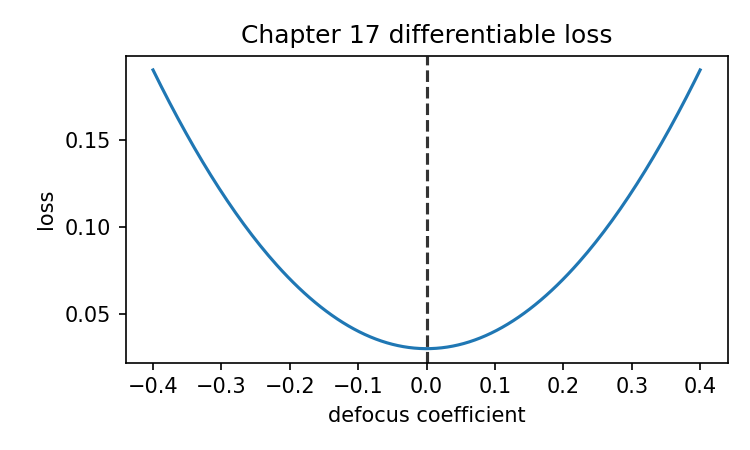
The optimizer should push the defocus coefficient toward a value that increases central PSF energy, typically toward reducing defocus.

This is a tiny example, but it is important because the whole path is differentiable:

phase coefficient
→ pupil phase
→ FFT field
→ PSF
→ center intensity loss
→ gradient
→ phase coefficient update

This is the style of computation that makes modern differentiable optics attractive.

We are no longer limited to optimizing only ray intercepts or simple scalar operands. We can optimize through image formation calculations.

13. End-to-end computational imaging

Classical lens design often treats the lens as the main object.

Modern computational imaging often treats the whole imaging system as the object:

scene
→ optics
→ sensor
→ noise
→ image processing
→ final image or task loss

In an end-to-end differentiable pipeline, some or all of these stages may be differentiable.

That allows a very different kind of optimization.

Instead of asking only:

Does the lens have high MTF?

we can ask:

Does the whole imaging system produce the best final result
after optics, sensor sampling, noise, and reconstruction?

For example, a computational camera may intentionally use an optical element that produces a PSF that looks strange by classical standards, because a reconstruction algorithm can decode it well.

A wavefront coding system may deliberately make the PSF less focus-sensitive.

A metasurface or diffractive optical element may be designed together with a neural reconstruction network.

A lens and image-processing model may be trained together for a specific task.

This is where differentiable optics becomes especially important.

If the whole pipeline is differentiable, we can compute gradients from the final loss all the way back to optical parameters.

The chain becomes:

final image loss
→ reconstruction algorithm
→ sensor model
→ PSF or wave optics model
→ optical parameters

That is end-to-end optimization.

But this power comes with a warning.

If the simulation is unrealistic, the optimized system may perform well in simulation and poorly in reality.

This is sometimes called a simulation-to-reality gap.

For optics, the gap can come from:

inaccurate material models;
manufacturing errors;
alignment tolerances;
temperature effects;
sensor noise assumptions;
diffraction model simplifications;
polarization effects;
stray light;
coating behavior;
imperfect calibration;
reconstruction model assumptions.

Differentiability does not remove these problems. It can even hide them behind beautiful training curves.

A careful statement is:

End-to-end differentiable optimization is only as trustworthy as the physical model and loss function it optimizes.

That sentence should stay close whenever the method looks magical.

14. Classical metrics still matter

Differentiable optics can optimize directly for image loss, task loss, or learned perceptual metrics.

That does not make classical optical metrics obsolete.

Spot diagrams, wavefront maps, PSF, MTF, distortion, field curvature, and tolerance analysis still matter because they reveal physical behavior.

A neural reconstruction metric may say the final image looks good, while the optical system has:

severe field-dependent blur;
high sensitivity to focus;
fragile alignment;
poor color behavior;
unacceptable distortion;
low light efficiency;
strong artifacts outside the training distribution.

Classical metrics are not old furniture to throw away.

They are diagnostic instruments.

A good modern workflow may include both:

classical optical metrics
+
differentiable end-to-end losses

The classical metrics tell us what the optics are doing.

The end-to-end loss tells us how the whole imaging system performs for a specific task.

Those are related but not identical.

This is a mature way to think about differentiable optics:

It expands the design space.
It does not cancel the need to understand optics.

15. Differentiable does not mean physically free

Gradient-based optimization can find surprising designs.

That can be good.

It can also create designs that are hard to manufacture, align, or interpret.

For example, if a phase mask is represented by free pixels, the optimizer may create a highly oscillatory phase pattern. It may perform well in simulation but be impossible to fabricate or too sensitive to wavelength.

If an aspheric surface has many free coefficients, the optimizer may create a surface with large slope changes or difficult testing requirements.

If a material parameter is allowed to vary continuously, the optimizer may choose a refractive index that does not correspond to any real glass.

So the parameterization matters.

A parameterization is how we describe the design variables.

Examples:

surface radii
conic constants
aspheric coefficients
Zernike phase coefficients
freeform surface coefficients
diffractive zone heights
pixelated phase mask values
glass interpolation variables
mechanical spacings

A good parameterization gives the optimizer freedom where freedom is useful and restriction where restriction is necessary.

This is another form of design judgment.

The optimizer follows gradients. It does not know which shapes are manufacturable unless manufacturability appears in the model or constraints.

16. Stable parameterization: an example

Suppose we want to optimize a phase mask.

A tempting parameterization is:

one free phase value per pixel

That gives enormous freedom.

It also allows noisy, rapidly varying patterns.

A smoother alternative is to represent the phase as a sum of low-order polynomial or Zernike-like terms:

$\phi(\rho,\theta) = a_1 Z_1(\rho,\theta) + a_2 Z_2(\rho,\theta) + \cdots + a_k Z_k(\rho,\theta)$

Now the trainable variables are coefficients:

$a_1, a_2, \ldots, a_k$

This reduces freedom but improves stability and interpretability.

In code, a simple defocus-plus-astigmatism phase model might be:

def phase_model(rho, theta, coeffs):
    """
    Simple differentiable phase model.

    coeffs[0] : defocus-like term
    coeffs[1] : astigmatism-like term
    coeffs[2] : coma-like teaching term
    """
    defocus = coeffs[0] * (2.0 * rho**2 - 1.0)
    astig = coeffs[1] * rho**2 * torch.cos(2.0 * theta)
    coma = coeffs[2] * (3.0 * rho**3 - 2.0 * rho) * torch.cos(theta)

    return defocus + astig + coma

This is not a full Zernike implementation, but it shows the idea.

The optimizer changes a few meaningful coefficients instead of thousands of unrelated pixels.

That often makes the problem easier and the result more understandable.

A good rule is:

Give the optimizer variables that describe plausible optical changes.

Not merely variables that are easy to put in a tensor.

17. A differentiable loss is a design statement

In Chapter 15, we said a merit function is a design argument.

The same is true here.

A differentiable loss tells the optimizer what matters.

If the loss maximizes PSF center intensity, the optimizer will try to concentrate energy at the center.

If the loss targets MTF at selected frequencies, it will try to improve those frequencies.

If the loss compares a reconstructed image to a ground truth image, it will try to improve that reconstruction.

If the loss is a neural-network task loss, it may optimize for classification or detection performance rather than human visual quality.

None of these is universally right.

The loss must match the imaging task.

For example:

A barcode scanner does not need the same optical priorities as a portrait lens.
A microscope does not need the same priorities as a phone camera.
A star tracker does not need the same priorities as an endoscope.

Differentiable optics does not remove the need to define the task.

It makes the task definition more direct and more consequential.

18. Gradient descent can be fooled

A gradient tells us a local direction.

It does not guarantee a globally best design.

Gradient descent can still suffer from:

local minima;
flat regions;
bad scaling;
unstable learning rates;
poor parameterization;
unrealistic losses;
constraints not represented in the model;
sensitivity to initialization.

For example, if the learning rate is too high, optimization may oscillate or diverge.

If the learning rate is too low, it may barely move.

If the initial design is physically poor, rays may miss surfaces or hit invalid regions.

If the loss landscape has many valleys, the optimizer may settle into a local compromise.

So the old lesson remains:

Optimization is a tool, not a guarantee.

Differentiability gives better information. It does not give wisdom.

19. Scaling still matters

Gradients depend on scale.

If one parameter is measured in millimeters and another is a tiny curvature in inverse millimeters, their gradient magnitudes may differ wildly.

If one loss term has values around 1000 and another around 0.001, the large term may dominate.

So differentiable optics still needs:

normalized variables;
normalized losses;
reasonable weights;
stable units;
bounded parameters;
good initialization.

This connects directly to Chapter 14.

Sampling and normalization did not stop mattering because we moved into PyTorch.

They matter more, because the gradients depend on them.

A wrong frequency axis in an MTF loss means the optimizer improves the wrong frequency.

A wrong PSF normalization means the gradient may reward energy scaling instead of image concentration.

A wrong aperture mask means the optimizer designs for the wrong physical system.

The safe chain is:

correct computation
→ correct loss
→ meaningful gradient
→ useful optimization

Do not skip the first two steps.

20. How differentiable optics connects to Optiland

A modern open optical design framework can be valuable in two ways.

First, it can provide classical analysis:

ray tracing
spot diagrams
wavefront
PSF
MTF
optimization

Second, if it supports differentiable or machine-learning-oriented workflows, it can help connect optical models with tensor libraries and gradient-based optimization.

A differentiable workflow outline looks like this:

# Version-checked workflow outline.
# Check the installed Optiland version and companion repository
# for exact API names.

# 1. Build or load an optical system.
# optic = make_system(...)

# 2. Select differentiable backend or tensor mode if supported.
# optic.enable_differentiable_backend("torch")

# 3. Mark parameters as trainable.
# optic.surface(1).radius.requires_grad = True
# optic.surface(2).radius.requires_grad = True
# optic.image_plane.position.requires_grad = True

# 4. Trace rays or compute wave optics result.
# result = optic.trace(...)

# 5. Compute loss.
# loss = result.rms_spot() + mtf_penalty(...)

# 6. Backpropagate.
# loss.backward()

# 7. Optimizer updates parameters.
# optimizer.step()

The exact API may differ. The structure is the important part.

What matters is that optical parameters participate in a differentiable computational graph.

The book’s earlier chain still applies:

surfaces
→ rays
→ wavefront
→ PSF
→ MTF

The differentiable addition is:

loss
→ gradients back through the chain
→ parameter updates

So differentiable optics is not a separate universe. It is the same computation chain with gradients attached.

21. Why open tools matter here

The educational value of open tools becomes especially clear in differentiable optics.

If a tool gives only a final result, you can use the result but cannot easily inspect the computational graph.

If a tool exposes the system as code, you can ask:

Which parameters require gradients?
Which operations are differentiable?
Where are masks or hard branches used?
Which loss is being optimized?
How are rays sampled?
How are invalid rays handled?
How is the PSF normalized?
How is the MTF frequency axis defined?
Which parameters actually changed?

This is not about worshiping open source.

It is about inspectability.

The sharper version of the claim is:

For learning differentiable optics, inspectability is not a luxury.
It is part of understanding the method.

A differentiable pipeline can be even more opaque than a classical one if all you see is a training loss curve.

Open, inspectable code helps prevent that.

22. A small gradient inspection habit

When doing differentiable optics, inspect gradients.

Not every step, not forever, but often enough to catch problems.

For example:

loss.backward()

print("c1 grad:", c1.grad)
print("c2 grad:", c2.grad)
print("z_image grad:", z_image.grad)

Ask:

Are the gradients finite?
Are they extremely large?
Are they exactly zero?
Do they change sign when expected?
Are some variables not receiving gradients?

If a variable has no gradient, perhaps it is not connected to the loss.

If gradients are nan, perhaps a square root, division, invalid ray, or normalization failed.

If gradients are huge, scaling may be poor.

If gradients are tiny, the problem may be flat, saturated, or badly scaled.

This is the differentiable version of inspecting intermediate optical plots.

Just as we inspected pupil amplitude and PSF centering, we inspect gradient health.

A practical debugging checklist:

[ ] Is the loss finite?
[ ] Are gradients finite?
[ ] Do trainable variables actually affect the loss?
[ ] Are units and scaling reasonable?
[ ] Are masks blocking gradients?
[ ] Are hard thresholds creating dead regions?
[ ] Does a small manual parameter change affect the loss as expected?

This saves time.

23. Differentiable optics and MTF: a careful example

Suppose we want to improve MTF at a selected frequency.

A naive loss might be:

loss = -mtf[fy, fx]

This maximizes one MTF sample.

That may work as a toy example, but in real design it is too narrow.

It can encourage the system to improve one point while ignoring nearby frequencies or other fields.

A better teaching loss might average over a small frequency band:

def band_mtf_loss(mtf, fy_slice, fx_slice, target=0.4):
    band = mtf[fy_slice, fx_slice]

    mean_mtf = torch.mean(band)

    error = torch.relu(target - mean_mtf)

    return error**2

A still better design loss may include:

multiple fields
multiple wavelengths
multiple frequency bands
geometry penalties
distortion penalties
manufacturing constraints

The differentiable method gives us gradients. It does not choose a wise loss automatically.

The design question remains:

Which image qualities matter for this system?

That question cannot be delegated to autodiff.

24. Differentiable rendering and learned reconstruction

In computational imaging, the optical system may be optimized together with reconstruction software.

A simplified training loop might look like this:

ground truth image
→ optical simulation
→ sensor simulation
→ reconstruction model
→ reconstructed image
→ loss against ground truth
→ gradients update optics and reconstruction parameters

In code structure:

# Conceptual structure only.

for image in training_images:
    optimizer.zero_grad()

    psf = optical_model(trainable_optical_parameters)

    sensor_image = simulate_sensor(image, psf, noise_model)

    reconstructed = reconstruction_model(sensor_image)

    loss = image_loss(reconstructed, image)

    loss.backward()

    optimizer.step()

This is much broader than classical lens optimization.

The loss may not be RMS spot or MTF. It may be:

mean squared image error;
perceptual loss;
classification loss;
detection loss;
depth estimation loss;
task-specific reconstruction loss.

This is why differentiable optics matters for modern imaging.

The optical design can be optimized for the final use of the image, not only for classical intermediate metrics.

But again, this is powerful and risky.

If the training images are not representative, the optical system may overfit.

If the sensor model is too clean, the design may fail with real noise.

If manufacturing variation is ignored, the design may be fragile.

If the reconstruction network is too powerful, it may hide optical weaknesses in simulation while producing artifacts in reality.

The more end-to-end the optimization becomes, the more careful the physical validation must be.

25. Validation does not disappear

A differentiable design still needs validation outside the training loop.

For a lens or computational camera, validation may include:

classical optical analysis
independent ray tracing
PSF and MTF checks
tolerance analysis
manufacturing constraints
sensor sampling checks
noise robustness
field and wavelength sweeps
test images outside the training set
physical prototype measurements

If a design only works under the exact differentiable simulation used to train it, it is not yet a robust optical design.

This is a healthy way to view differentiable optics:

Use differentiability to search.
Use optical analysis to understand.
Use validation to trust.

All three are needed.

26. Why this matters to the reader of this book

This book has spent many chapters unpacking classical calculations.

That was not a detour.

It is the foundation needed to understand differentiable optics.

If someone says:

We optimize the lens end to end through a differentiable imaging pipeline.

you can now ask:

What is the optical model?
Does it trace real rays or use paraxial approximations?
Does it include diffraction?
How is the pupil function represented?
How is the PSF computed?
Is the sensor model included?
What loss is optimized?
Which optical parameters are trainable?
Are materials discrete or continuous?
How are apertures and vignetting handled?
Are gradients stable?
What classical metrics were checked afterward?

These are not skeptical questions for their own sake.

They are the questions needed to understand the claim.

Differentiable optics is exciting precisely because it extends the chain we have already built. Without that chain, it is only another black box.

27. A small side-by-side comparison

It may help to compare three optimization styles.

Style	What it needs	Strength	Risk
Derivative-free search	Merit values	Simple to use; can handle awkward functions	Can be slow; may need many evaluations
Classical gradient / least-squares optimization	Merit and derivative-like information	Efficient for smooth optical design problems	Depends on scaling, local behavior, operand design
Autodiff differentiable optics	Differentiable computational graph	Can optimize through rays, waves, sensors, and reconstruction	Requires careful differentiable modeling and validation

None is universally best.

A small lens design problem may work well with traditional optical optimization.

A wavefront-coded computational camera may benefit from end-to-end differentiable optimization.

A rugged engineering design may still need classical tolerance analysis and human review.

The practical lesson is:

Choose the optimization method to match the problem,
not because one method sounds more modern.

28. The main conceptual upgrade

The main upgrade in this chapter is not “use PyTorch.”

The main upgrade is this:

Optical computation can become part of a differentiable program.

Once that happens, optical variables can be optimized together with other differentiable components.

The lens can be connected to:

phase masks;
diffractive elements;
sensor models;
reconstruction algorithms;
neural networks;
task-specific losses.

This is why differentiable optics is important.

It changes the boundary of the design problem.

Classical design often asks:

What lens gives good optical metrics?

Differentiable computational imaging may ask:

What optical system and computational reconstruction together give the best final result?

That is a larger question.

It is also a more dangerous question if asked carelessly.

The larger the optimization loop, the more important it is to understand every link in the chain.

29. What not to believe

Because differentiable optics is connected to machine learning, it is easy for exaggerated claims to appear.

Be cautious with claims like:

The network will learn the optics.
The optimizer will discover the best lens.
Physics constraints are no longer necessary.
MTF is obsolete.
Classical optical design is dead.

These claims are too loose.

A better view is:

Differentiable optimization can search design spaces that are hard to explore manually.
But the result still depends on physical modeling, constraints, losses, data, and validation.

That view keeps the excitement without losing judgment.

This book’s position is not anti-modern. It is anti-mystification.

Differentiable optics is worth learning because it is powerful.

It is also worth demystifying because it is powerful.

30. Preparing for the final chapter

We are now ready to return to the reader’s practical task.

At the beginning of the book, the question was:

Where does an MTF curve come from?

We have answered that.

Now a new question appears:

When optical software gives me any output,
how should I read it?

This includes classical outputs:

layout;
prescription;
spot diagram;
ray fan;
OPD;
PSF;
MTF;
merit value.

It also includes modern outputs:

gradient;
training loss;
optimized phase mask;
differentiable ray trace result;
end-to-end reconstruction score.

The same habit applies:

Do not stop at the output.
Trace the computation that produced it.

That habit is the real skill this book has been teaching.

The final chapter will collect that skill into a practical reading checklist.

Chapter summary

Differentiable optics means building optical computations so that gradients can be computed with respect to design parameters.

Automatic differentiation applies the chain rule through executed operations. It is different from manually estimating derivatives by finite differences.

A differentiable optical chain may look like:

optical parameters
→ ray tracing or wave optics
→ PSF / MTF / image simulation
→ loss
→ gradients
→ parameter update

PyTorch examples show the basic pattern:

define trainable variables
compute optical result
compute loss
call backward()
update variables

Differentiable ray tracing extends ordinary ray tracing by allowing derivatives to flow through intersections, normals, refraction, propagation, and image-plane errors.

Differentiable PSF and MTF calculations can be built with tensor FFT operations, allowing losses based on image formation or frequency response.

The method is powerful for modern computational imaging because optics, sensors, reconstruction algorithms, and task losses can be optimized together.

But differentiable optics is not magic. It still needs correct physics, stable sampling, meaningful losses, good parameterization, constraints, manufacturability checks, and validation outside the training loop.

The central idea is:

Differentiable optics does not replace the classical computation chain.
It attaches gradients to that chain.

That makes the chain more powerful, but also makes understanding it more important.

Generated validation figure

Differentiable loss curve generated from the Chapter 17 gradient-descent check

Source and validation note

This chapter is an orientation chapter, not a survey of the entire differentiable-optics literature. The retained claim is limited: automatic differentiation can attach gradients to optical computation chains when the operations are implemented in differentiable numerical frameworks. Practical design still requires physical modeling, constraints, sampling checks, and validation outside the training loop.

Keyboard shortcuts

Computational Optics